Artificial
Intelligence 3E
foundations of computational agents
3.5 Uninformed Search Strategies
A problem determines the graph, the start node, and the goal but not which path to select from the frontier. This is the job of a search strategy. A search strategy defines the order in which paths are selected from the frontier. It specifies which path is selected at line 13 of Figure 3.5. Different strategies are obtained by modifying how the selection of paths in the frontier is implemented.
This section presents four uninformed search strategies that do not take into account the location of the goal. Intuitively, these algorithms ignore where they are going until they find a goal and report success.
3.5.1 Breadth-First Search
In breadth-first search the frontier is implemented as a FIFO (first-in, first-out) queue. Thus, the path that is selected from the frontier is the one that was added earliest. The paths from the start node are generated in order of the number of arcs in the path. One of the paths with the fewest arcs is selected at each iteration.
Example 3.8.
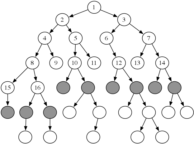
Consider the tree-shaped graph in Figure 3.6. Suppose the start node is the node at the top, and the children of a node are added in a left-to-right order. In breadth-first search, the order in which the paths are expanded does not depend on the location of the goal. The nodes at the end of the first 16 paths expanded are numbered in order of expansion in the figure. The shaded nodes are the nodes at the ends of the paths on the frontier after the first 16 iterations.
Example 3.9.
Consider breadth-first search from in the graph given in Figure 3.3. The costs are ignored in breadth-first search, so it is searching in the space without weights, as shown in Figure 3.7.
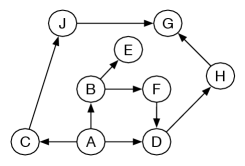
Initially, the frontier is . This is extended by ’s neighbors, making the frontier , , . These are the paths of length one starting at . The next three paths expanded are , , and , after which the frontier is
These are the paths of length two starting at . These are the next paths expanded, at which stage the frontier contains the paths of length three from , namely
When is selected, it is returned as a solution.
In breadth-first search, each path on the frontier has either the same number of arcs as, or one more arc than, the next path on the frontier that is expanded.
Suppose the branching factor of the search is . If the next path to be selected on the frontier contains arcs, there are at least elements of the frontier. All of these paths contain or arcs. Thus, both space and time complexities to find a solution are exponential in the number of arcs of the path to a goal with the fewest arcs. This method is guaranteed to find a solution if one exists and will find a solution with the fewest arcs.
Breadth-first search is useful when
-
•
the problem is small enough so that space is not a problem, such as when the graph is already stored, and
-
•
a solution containing the fewest arcs is required.
It is a poor method when all solutions have many arcs or there is some heuristic knowledge available. It is not used very often for large problems where the graph is dynamically generated because of its exponential space complexity.
3.5.2 Depth-First Search
In depth-first search, the frontier acts like a LIFO (last-in, first-out) stack of paths. In a stack, elements are added and removed from the top of the stack. Using a stack means that the path selected and removed from the frontier at any time is the last path that was added.
Example 3.10.
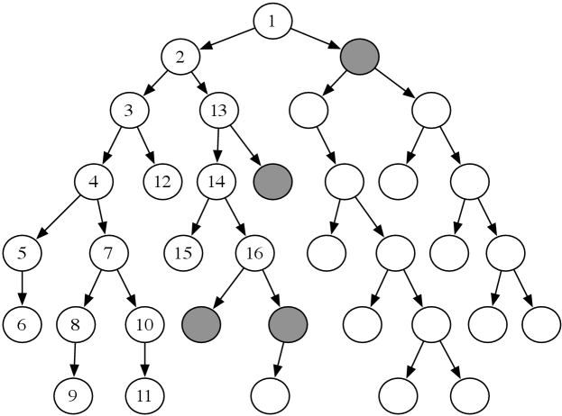
Consider the tree-shaped graph in Figure 3.8. Suppose the start node is the root of the tree (the node at the top). As depth-first search does not define the order of the neighbors, suppose for this graph that the children of each node are ordered from left to right, and are added to the stack in reverse order so that the path to the leftmost neighbor is added to the stack last (and so removed first).
In depth-first search, like breadth-first search, the order in which the paths are expanded does not depend on the goal. The nodes at the end of the first 16 paths expanded are numbered in order of expansion in Figure 3.8. The shaded nodes are the nodes at the ends of the paths on the frontier after the first 16 steps, assuming none of the expanded paths end at a goal node.
The first six paths expanded, , , , , , and , are all initial parts of a single path. The node at the end of this path (node 6) has no neighbors. The seventh path expanded is . The next path expanded after path always contains an initial segment of path with one extra node.
Implementing the frontier as a stack results in paths being pursued in a depth-first manner – searching one path to its completion before trying an alternative path. This method is said to involve backtracking: the algorithm selects a first alternative at each node, and it backtracks to the next alternative when it has pursued all of the paths from the first selection. Some paths may be infinite when the graph has cycles or infinitely many nodes, in which case a depth-first search may never stop.
This algorithm does not specify the order in which the paths to the neighbors are added to the frontier. The efficiency of the algorithm can be sensitive to the order in which the neighbors are expanded.
Figure 3.9 shows an alternative implementation of depth-first search that uses recursion to implement the stack. The call , if it halts, returns a path from node to a goal node, or if there is no path. Backtracking is achieved by the recursive call returning and the next neighbor being explored.
Example 3.11.
Consider depth-first search from to in the graph of Figure 3.3. In this example, the frontier is shown as a list of paths with the top of the stack at the left of the list. The ordering of the neighbors matters; assume that the neighbors are ordered so they are expanded in alphabetic ordering.
Initially, the frontier is .
At the next stage, the frontier contains the paths
Next, the path is selected because it is at the top of the stack. It is expanded, giving the frontier
Next, the path is removed. has no neighbors, and so no paths are added. The resulting frontier is
At this stage, the path is expanded, resulting in the frontier
The next frontiers are
The path is selected from the frontier and returned as the solution found.
Suppose is the path selected on line 13 of Figure 3.5. In depth-first search, every other path on the frontier is of the form , for some index and some node that is a neighbor of ; that is, it follows the selected path for a number of arcs and then has exactly one extra node. Thus, the frontier contains only the current path and paths to neighbors of the nodes on this path. If the branching factor is and the selected path, , on the frontier has arcs, there can be at most other paths on the frontier. These paths all follow an initial segment of path , and have one extra node, a neighbor of a node in path , and there are at most neighbors from each node. Therefore, for depth-first search, the space used at any stage is linear in the number of arcs from the start to the current node.
Comparing Algorithms
Algorithms (including search algorithms) can be compared on
-
•
the time taken
-
•
the space used
-
•
the quality or accuracy of the results.
The time taken, space used, and accuracy of an algorithm are a function of the inputs to the algorithm. Computer scientists talk about the asymptotic complexity of algorithms, which specifies how the time or space grows with the input size of the algorithm. An algorithm has time (or space) complexity – read “big-oh of ” – for input size , where is some function of , if there exist constants and such that the time, or space, of the algorithm is less than for all . The most common types of functions are exponential functions such as , , or ; polynomial functions such as , , , or ; and logarithmic functions, . In general, exponential algorithms get worse more quickly than polynomial algorithms which, in turn, are worse than logarithmic algorithms.
An algorithm has time or space complexity for input size if there exist constants and such that the time or space of the algorithm is greater than for all . An algorithm has time or space complexity if it has complexity and . Typically, you cannot give a complexity on an algorithm, because most algorithms take different times for different inputs. Thus, when comparing algorithms, one has to specify the class of problems that will be considered.
Saying algorithm is better than , using a measure of either time, space, or accuracy, could mean any one of:
-
•
the worst case of is better than the worst case of
-
•
works better in practice, or the average case of is better than the average case of , where you average over typical problems
-
•
there is a subclass of problems for which is better than , so which algorithm is better depends on the problem
-
•
for every problem, is better than .
The worst-case asymptotic complexity is often the easiest to show, but it is usually the least useful. Characterizing the subclass of problems for which one algorithm is better than another is usually the most useful, if it is easy to determine which subclass a given problem is in. Unfortunately, this characterization is usually very difficult to obtain.
Characterizing when one algorithm is better than the other can be done either theoretically using mathematics or empirically by building implementations. Theorems are only as valid as the assumptions on which they are based. Similarly, empirical investigations are only as good as the suite of test cases and the actual implementations of the algorithms. It is easy to disprove a conjecture that one algorithm is better than another for some class of problems by showing a counterexample, but it is usually much more difficult to prove such a conjecture.
If there is a solution on the first branch searched, the time complexity is linear in the number of arcs in the path. In the worst case, depth-first search can get trapped on infinite branches and never find a solution, even if one exists, for infinite graphs or for graphs with cycles. If the graph is a finite tree, with the forward branching factor less than or equal to and with all paths from the start having or fewer arcs, the worst-case time complexity is .
Example 3.12.
Consider the delivery graph presented in Figure 3.10, in which the agent has more freedom in moving between locations, but can get into cycles. An infinite path leads from to to and back to . Depth-first search may follow this path forever, never considering alternative paths. If the neighbors are selected in alphabetic ordering, the frontiers for the first few iterations of depth-first search from are
Depth-first search will never halt for this example. The last three paths are never explored.
Because depth-first search is sensitive to the order in which the neighbors are added to the frontier, care must be taken to do it sensibly. This ordering may be done statically (so that the order of the neighbors is fixed) or dynamically (where the ordering of the neighbors depends on the goal).
Depth-first search is appropriate when
-
•
space is restricted
-
•
many solutions exist, perhaps with long paths, particularly for the case where nearly all paths lead to a solution, or
-
•
the order in which the neighbors of a node are added to the stack can be tuned so that solutions are found on the first try.
It is a poor method when
-
•
it is possible to get caught in infinite paths, which occurs when the graph is infinite or when there are cycles in the graph
-
•
solutions exist at shallow depth, because in this case the search may explore many long paths before finding the short solutions, or
-
•
there are multiple paths to a node, for example, on an grid, where all arcs go right or down, there are exponentially many paths from the top-left node, but only nodes.
Depth-first search is the basis for a number of other algorithms, including iterative deepening, described next.
3.5.3 Iterative Deepening
Neither of the preceding methods is ideal. Breadth-first search, which guarantees that a path will be found, requires exponential space. Depth-first search may not halt on infinite graphs or graphs with cycles. One way to combine the space efficiency of depth-first search with the optimality of breadth-first search is to use iterative deepening. The idea is to recompute the elements of the breadth-first frontier rather than storing them. Each recomputation can be a depth-first search, which thus uses less space.
Iterative deepening repeatedly calls a depth-bounded searcher, a depth-first searcher that takes in an integer depth bound and never explores paths with more arcs than this depth bound. Iterative deepening first does a depth-first search to depth 1 by building paths of length 1 in a depth-first manner. If that does not find a solution, it can build paths to depth 2, then depth 3, and so on until a solution is found. When a search with depth bound fails to find a solution, it can throw away all of the previous computation and start again with a bound of . Eventually, it will find a solution if one exists, and, as it is enumerating paths in order of the number of arcs, a path with the fewest arcs will always be found first.
To ensure it halts for finite graphs, iterative deepening search needs to distinguish between
-
•
failure because the depth bound was reached
-
•
failure due to exhausting the search space.
In the first case, the search must be retried with a larger depth bound. In the second case, it is a waste of time to try again with a larger depth bound, because no path exists no matter what the depth, and so the whole search should fail.
Pseudocode for iterative deepening search, , is presented in Figure 3.11. The local procedure implements a depth-bounded depth-first search, using recursion to keep the stack, similar to Figure 3.9, but with a limit on the length of the paths for which it is searching. It finds paths of length , where is the path length of the given path from the start and is a non-negative integer.
The iterative deepening searcher calls for increasing depth bounds. only needs to check for a goal when , because it is only called when there are no solutions for lower bounds. explores the paths to goal nodes in the same order as breadth-first search, but regenerates the paths.
To ensure that iterative deepening search fails whenever breadth-first search would fail, it needs to keep track of when increasing the bound could help find an answer. A depth-bounded search fails naturally – it fails by exhausting the search space – if the search did not prune any paths due to the depth bound. In this case, the program can stop and report no paths. This is handled through the variable , which is false when is called initially, and becomes true if the search is pruned due to the depth bound. If it is true at the end of a depth-bounded search, the search failed due to hitting the depth bound, and so the depth bound can be increased, and another depth-bounded search is carried out.
The obvious problem with iterative deepening is the wasted computation that occurs at each step. This, however, may not be as bad as one might think, particularly if the branching factor is high. Consider the running time of the algorithm. Assume a constant branching factor of . Consider the search where the bound is . At depth , there are nodes; each of these has been generated once. The nodes at depth have been generated twice, those at depth have been generated three times, and so on, and the nodes at depth have been generated times. Thus, the total number of paths expanded is
Breadth-first search expands nodes. Thus, iterative deepening has an asymptotic overhead of times the cost of expanding the paths at depth using breadth-first search. Thus, when there is an overhead factor of , and when there is an overhead of . This algorithm is and there cannot be an asymptotically better uninformed search strategy. Note that, if the branching factor is close to one, this analysis does not work because then the denominator would be close to zero; see Exercise 3.9.
3.5.4 Lowest-Cost-First Search
For many domains, arcs have non-unit costs, and the aim is to find an optimal solution, a solution such that no other solution has a lower cost. For example, for a delivery robot, the cost of an arc may be resources (e.g., time, energy) required by the robot to carry out the action represented by the arc, and the aim is for the robot to solve a given goal using fewest resources. The cost for a tutoring agent (Example 3.5) may be the time and effort required by a student. In each of these cases, the searcher should try to minimize the cost of the path found to a goal.
The search algorithms considered thus far are not guaranteed to find the minimum-cost paths; they have not used the arc cost information at all. Breadth-first search finds a solution with the fewest arcs first, but the distribution of arc costs may be such that a path with the fewest arcs is not one of minimal cost.
The simplest search method that is guaranteed to find a minimum-cost path is lowest-cost-first search (also called least-cost search or uniform-cost search), which is similar to breadth-first search, but instead of expanding a path with the fewest number of arcs, it selects a path with the lowest cost. This is implemented by treating the frontier as a priority queue ordered by the function.
Example 3.13.
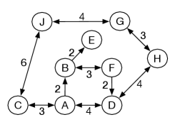
Consider lowest-cost-first search from to in the running example of the delivery graph given in Figure 3.3. In this example, paths are shown with a subscript showing the cost of the path. The frontier is shown as a list of paths in order of cost.
Initially, the frontier is . At the next stage it is . The path is expanded, with the resulting frontier
The path is then expanded, resulting in the frontier
Next, the path is expanded. has no neighbors, so the path is removed. Next, the path is expanded, resulting in the frontier
Then the path to is expanded, resulting in the frontier
Then the path is expanded, and the resulting frontier is
The path is expanded, giving
The path is expanded, and then, depending on the order that ties are broken, the path is selected and returned as the solution, either next or the step after.
If the costs of the arcs are all greater than a positive constant, known as bounded arc costs, and the branching factor is finite, the lowest-cost-first search is guaranteed to find an optimal solution – a solution with lowest path cost – if a solution exists. Moreover, the first path to a goal that is expanded is a path with lowest cost. Such a solution is optimal, because the algorithm expands paths from the start node in order of path cost, and the path costs never decrease as arc costs are positive. If a better path to a goal existed than the first solution found, it would have been expanded from the frontier earlier.
The bounded arc cost is used to guarantee the lowest-cost search will find a solution, when one exists, in graphs with finite branching factor. Without such a bound there can be infinite paths with a finite cost. For example, there could be nodes with an arc for each with cost . Infinitely many paths of the form all have a cost of less than 1. If there is an arc from to a goal node with a cost equal to 1, it will never be selected. This is the basis of Zeno’s paradox that Aristotle wrote about more than 2300 years ago.
Suppose that all arc costs are greater than or equal to . Let be the maximum branching factor, the cost of a lowest-cost path to a goal, and . is the maximum number of steps in a path that need to be considered in the search before finding a goal. In the worst case, the complexity for both space and time is , as there may need to be paths explored where each path is of length . It generates all paths from the start that have a cost less than the cost of a solution, and some of the paths that are of the cost of a solution, until it finds a path that is a solution.
Artificial Intelligence: Foundations of Computational Agents, Poole
& Mackworth
Copyright © 2023, David L. Poole and Alan K. Mackworth. 
This work is licensed under a Creative Commons Attribution-NonCommercial-NoDerivatives 4.0 International License.