Artificial
Intelligence 3E
foundations of computational agents
3.12 Exercises
Exercise 3.1.
Consider the graph of Figure 3.20, where the problem is to find a path from start to goal .
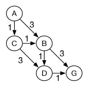
For each of the following algorithms, show the sequence of frontiers and give the path found.
-
(a)
Depth-first search, where the neighbors are expanded in alphabetic ordering
-
(b)
Breadth-first search
-
(c)
Lowest-cost-first search ( with for all nodes )
-
(d)
with (the -distance plus -distance from to ), where , , , , , , , , , and .
Exercise 3.2.
Consider the problem of finding a path in the grid shown in Figure 3.21 from the position to the position . A piece can move on the grid horizontally or vertically, one square at a time. Each step has cost 1. No step may be made into a forbidden shaded area or outside the grid.

-
(a)
For the grid shown in Figure 3.21, number the nodes expanded (in order) for a depth-first search from to , given that the order of the operators is up, down, left, right. Assume there is cycle pruning. What is the first path found?
-
(b)
For the same grid, number the nodes expanded, in order, for a least-cost-first search with multiple-path pruning search from to (Dijkstra’s algorithm). What is the first path found?
-
(c)
Number the nodes in order for an search, with multiple-path pruning, for the same grid, where the heuristic value for node is Manhattan distance from to the goal. The Manhattan distance between two points is the distance in the -direction plus the distance in the -direction. It corresponds to the distance traveled along city streets arranged in a grid. What is the path found?
-
(d)
Show how to solve the same problem using dynamic programming. Give the value for each node, and show which path is found.
-
(e)
Based on this experience, discuss which algorithms are best suited for this problem.
-
(f)
Suppose that the grid extended infinitely in all directions. That is, there is no boundary, but , , and the blocks are in the same positions relative to each other. Which methods would no longer find a path? Which would be the best method, and why?
Exercise 3.3.
This question investigates using graph searching to design video presentations. Consider a database of video segments, together with their length in seconds and the topics covered:
| Segment | Length | Topics Covered |
|---|---|---|
| seg0 | 10 | [welcome] |
| seg1 | 30 | [skiing, views] |
| seg2 | 50 | [welcome, artificial_intelligence, robots] |
| seg3 | 40 | [graphics, dragons] |
| seg4 | 50 | [skiing, robots] |
In the search graph, a node is a pair
where is a list of segments that must be in the presentation, and is a list of topics that also must be covered.
The neighbors of a node are obtained by first selecting a topic from . There is a neighbor for each segment that covers the selected topic. The remaining topics are the topics not covered by the segment added. [Part of this exercise is to think about the exact structure of these neighbors.] Assume that the leftmost topic is selected at each step.
Given the above database, the neighbors of the node , when is selected, are and .
Thus, each arc adds exactly one segment but can cover (and so remove) one or more topics. Suppose that the cost of the arc is equal to the time of the segment added.
The goal is to design a presentation that covers all of the topics in the list . The starting node is . The goal nodes are of the form . The cost of the path from a start node to a goal node is the time of the presentation. Thus, an optimal presentation is a shortest presentation that covers all of the topics in .
-
(a)
Suppose that the goal is to cover the topics and the algorithm always selects the leftmost topic to find the neighbors for each node. Draw the search space expanded for a lowest-cost-first search until the first solution is found. This should show all nodes expanded, which node is a goal node, and the frontier when the goal was found.
-
(b)
Give a non-trivial heuristic function that is admissible. [Note that for all is the trivial heuristic function.] Does it satisfy the monotone restriction for a heuristic function?
-
(c)
Does the topic selected affect the result found? Why or why not?
Exercise 3.4.
Give two different admissible non-trivial heuristics for the video game of Example 3.3 (depicted in Figure 3.2). Is one always less than or equal to the other? Explain why or why not.
Exercise 3.5.
Draw two different graphs, indicating start and goal nodes, for which forward search is better in one and backward search is better in the other.
Exercise 3.6.
The algorithm does not define what happens when multiple elements on the frontier have the same -value. Compare the following tie-breaking conventions by first conjecturing which will work better, and then testing it on some examples. Try it on some examples where there are multiple optimal paths to a goal (such as finding a path from the bottom left of a rectangular grid to the top right of the grid, where the actions are step-up and step-right). Of the paths on the frontier with the same minimum -value, select one:
-
(i)
uniformly at random
-
(ii)
that has been on the frontier the longest
-
(iii)
that was most recently added to the frontier
-
(iv)
with the smallest -value
-
(v)
with the least cost.
The last two may require other tie-breaking conventions when the cost and values are equal.
Exercise 3.7.
Consider what happens if the heuristic function is not admissible, but is still non-negative. What guarantees can be made when the path found by when the heuristic function:
-
(a)
is less than times the least-cost path (e.g., is less than greater than the cost of the least-cost path)
-
(b)
is less than more than the least-cost path (e.g., is always no more than 10 units greater than the cost of the optimal path)?
Develop a hypothesis about what would happen and show it empirically or prove your hypothesis. Does it change if multiple-path pruning is in effect or not?
Does loosening the heuristic in either of these ways improve efficiency? Try search where the heuristic is multiplied by a factor , or where a cost is added to the heuristic, for a number of graphs. Compare these on the time taken (or the number of nodes expanded) and the cost of the solution found for a number of values of or .
Exercise 3.8.
How can depth-first branch and bound be modified to find a path with a cost that is not more than, say, greater than the least-cost path. How does this algorithm compare to from the previous question?
Exercise 3.9.
The overhead for iterative deepening with on the denominator is not a good approximation when . Give a better estimate of the complexity of iterative deepening when . [Hint: Think about the case when .] How does this compare with for such graphs? Suggest a way that iterative deepening can have a lower overhead when the branching factor is close to 1.
Exercise 3.10.
Bidirectional search must be able to determine when the frontiers intersect. For each of the following pairs of searches, specify how to determine when the frontiers intersect:
-
(a)
breadth-first search and depth-bounded depth-first search
-
(b)
iterative deepening search and depth-bounded depth-first search
-
(c)
and depth-bounded depth-first search
-
(d)
and .
Exercise 3.11.
The depth-first branch and bound of Figure 3.14 is like a depth-bounded search in that it only finds a solution if there is a solution with cost less than . Show how this can be combined with an iterative deepening search to increase the depth bound if there is no solution for a particular depth bound. This algorithm must return in a finite graph if there is no solution. The algorithm should allow the bound to be incremented by an arbitrary amount and still return an optimal (least-cost) solution when there is a solution.
Artificial Intelligence: Foundations of Computational Agents, Poole
& Mackworth
Copyright © 2023, David L. Poole and Alan K. Mackworth. 
This work is licensed under a Creative Commons Attribution-NonCommercial-NoDerivatives 4.0 International License.