Artificial
Intelligence 3E
foundations of computational agents
17.3 Learning Interdependence of Relations
17.3.1 Relational Probabilistic Models
An alternative to the previous models that learn embedding of entities and relations is to learn the interdependencies of relations, building models that predict some relations in terms of others, similar to how graphical models of Chapter 9 represented the interdependencies of random variables.
The belief networks of Chapter 9 were defined in terms of random variables. Many domains are best modeled in terms of entities and relations. Agents must often build models before they know what entities are in the domain and, therefore, before they know what random variables exist. When the probabilities are being learned, the probabilities often do not depend on the identity of the entities. Probability models with entities and relations are studied in the area of statistical relational AI, and the models are referred to as relational probabilistic models, probabilistic relational models, or probabilistic logic models.
Example 17.5.
Consider the problem of predicting how well students will do in courses they have not taken. Figure 17.3 shows some fictional data designed to show what can be done. Students and have a B average, on courses both of which have B averages. However, you should be able to distinguish them as you know something about the courses they have taken.
A relational probabilistic model (RPM) is a model in which the probabilities are specified on the relations, independently of the actual entities. The entities share the probability parameters. The sharing of the parameters is known as parameter sharing or weight tying, as in convolutional neural networks.
A parameterized random variable is of the form , where each is a term (a logical variable or a constant). The parameterized random variable is said to be parameterized by the logical variables that appear in it. A ground instance of a parameterized random variable is obtained by substituting constants for the logical variables in the parameterized random variable. The ground instances of a parameterized random variable correspond to random variables, as in Section 17.1. The domain of the random variable is the range of . A Boolean parameterized random variable corresponds to a predicate symbol. For example, is a parameterized random variable, and is a random variable with domain the set of all possible grades.
We use the Datalog convention that logical variables start with an upper-case letter and constants start with a lower-case letter. Parameterized random variables are written starting with an upper-case letter, with the corresponding proposition in lower case (e.g., is written as , and is written as ), similar to the convention for random variables.
A plate model consists of
-
•
a directed graph in which the nodes are parameterized random variables
-
•
a population of entities for each logical variable, and
-
•
a conditional probability of each node given its parents.
A rectangle – a plate – is drawn around the parameterized random variables that share a logical variable. There is a plate for each logical variable. This notation is redundant, as the logical variables are specified in both the plates and the arguments. Sometimes one of these is omitted; often the arguments are omitted when they can be inferred from the plates.
Example 17.6.
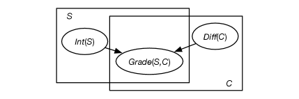
Figure 17.4 gives a plate model for predicting student grades. There is a plate for the courses and a plate for the students. The parameterized random variables are
-
•
, which represents whether student is intelligent
-
•
, which represents whether course is difficult,
-
•
, which represents the grade of student in course .
The probabilities for , , and need to be specified. If and are Boolean (with range and ) and has range , then there are 10 parameters that define the probability distribution. Suppose and and is defined by the following table:
Eight parameters are required to define because there are four cases, and each case requires two numbers to be specified; the third can be inferred to ensure the probabilities sum to one.
If there were students and courses, in the grounding there would be instances of , instances of , and instances of . So there would be random variables in the grounding.
A model that contains parametrized random variables is called a lifted model. A plate model means its grounding – the belief network in which nodes are all ground instances of the parameterized random variables (each logical variable replaced by an entity in its population) and the arcs are preserved. That is, the parametrized random variables in each plate are replicated for each entity. The conditional probabilities of the grounded belief network are the same as the corresponding instances of the plate model.
Example 17.7.
Consider conditioning the plate model of Figure 17.4 on the data given in Figure 17.3, and querying the random variables corresponding to the last two rows. There are 4 courses and 4 students, and so there would be 24 random variables in the grounding. All of the instances of that are not observed or queried can be pruned or never constructed in the first place, resulting in the belief network of Figure 17.5.
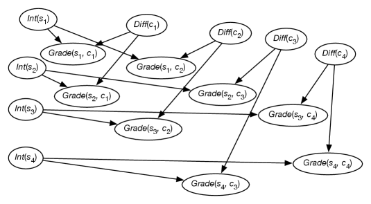
From this network, conditioned on the , the observed grades of Figure 17.3, and using the probabilities of Example 17.6, the following posterior probabilities can be derived:
Thus, this model predicts that is likely to do better than in course .
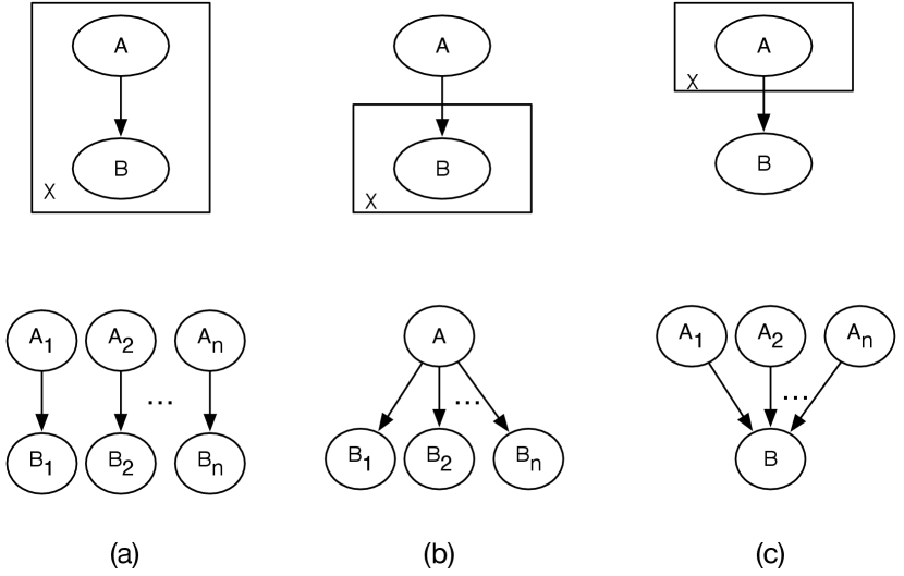
Figure 17.6 shows the three cases of how a directed arc interacts with a plate. The population of logical variable is . The random variable is written as , and similarly for . The parametrization can be inferred from the plates.
In Figure 17.6(a), and are both within the plate, and so represent the parametrized random variables and . In the grounding, the arc is replicated for every value of . The conditional probability is the same for every , and is the one modeled by in the lifted model. and are independent of and for , unless there is another arc to make them dependent.
In Figure 17.6(b), the parent is outside of the plate, and so it is not replicated for each element of the population. is the same for all . This makes the dependent on each other when is not observed. The number of parameters in the lifted models of Figure 17.6(a) and (b) is the same as the network without the plates, and so is independent of the population size .
In Figure 17.6(c), the child is outside of the plate, with a variable number of parents. In this case has parents and so cannot use the conditional probability . It needs an aggregator to compute the probability from arbitrary many parents. The aggregator is symmetric, as the index is of no significance; exchanging the names has no effect. This symmetry is called exchangeability. Some aggregators are the following:
-
•
If the model is specified as a probabilistic logic program with Boolean logical variables, the existential quantification of the logical variables in the body of a clause results in a noisy-or aggregation. In the aggregator of Figure 17.6(c), the noisy-or is equivalent to , where and are independent random variables for all instances of .
-
•
The model can be specified using weighted logical formulas, extended to first-order logic. A first-order weighted logical formula is a pair of a first-order logic formula and a weight. The conditional probability is proportional to the exponential of the sum of weights of the groundings of formulas that are true. In this case, the aggregation becomes a case of logistic regression, called relational logistic regression.
For example, the first-order weighted formulas , and result in , where is an assignment of values to the parents consisting of entities with and entities with .
-
•
Standard database aggregators such as average, sum, or max of some values of the parents can be used.
-
•
A more sophisticated aggregation, latent Dirichlet allocation (LDA), is when the population of the plate corresponds to the domain of the child. The value of can be used to compute . For example, using a softmax
(or perhaps without the exponentiation, if ). The aggregation is thus implementing an attention mechanism, similar to that used in transformers.
For overlapping plates, the values are duplicated for each plate separately, as in the following example.
Example 17.8.
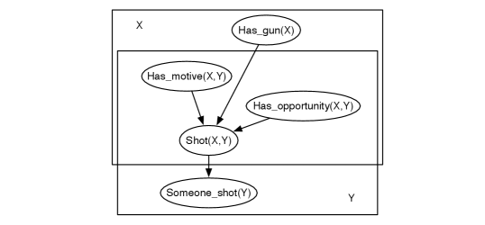
Suppose someone was shot and the problem is to determine who did it. Assume the shooting depends on having motive, opportunity, and a gun. A plate model for this is shown in Figure 17.7, where is the person shot and is the shooter.
When a particular person is observed to be shot, the aim is to determine which person could have shot them. The motive and the opportunity depend on both and , but whether the shooter, , has a gun does not depend on . Noisy-or is an appropriate aggregator here; is shot if there exists someone who shot them, but there is some chance they were shot even if no one shot them (e.g., a gun went off randomly). There are probably different probabilities for the cases where (they shot themself) and for (the shooter and victim were different people). If there are 1000 people, there are 3,002,000 random variables in the grounding, including a million instances of and a thousand instances of . If all of the variables are Boolean, there are 13 parameters to be assigned: eight for , two for , and one each for the other (parameterized) random variables. Each of these other variables could have parents; see Exercise 17.5.
17.3.2 Collective Classification and Crowd Sourcing
Suppose there are many true/false questions that you would like the answer to. One way to find the answer might be to ask many people using crowd sourcing, where the users might be paid for reliable answers. Each person answers some subset of the questions; the aim is to determine which questions are true, and who to pay. Some people and bots may give random answers, in the hope of being paid for very little work. The problem of determining truth from crowd sourcing is called truth discovery.
One application for truth discovery is to evaluate predictions of an AI algorithm on a knowledge graph. You cannot just use a held-out test set for evaluation as there are only positive examples in a knowledge graph. Negative examples are required to evaluate probabilistic predictions, for example, using log loss. Negative examples can be acquired by crowd sourcing.
One way to represent this problem is the plate model of Figure 17.8, where , the provided answer by user to question , depends on the reliability of and the truth of .
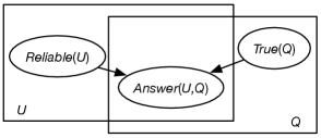
The conditional probabilities can specify that the answer provided by reliable users is highly likely to be the truth, and the answer provided by an unreliable person is likely to be random. When conditioned on the answers provided, the users are classified as reliable or not and the questions are classified as true or false. It may not take many reliable users answering a particular question to make us quite sure of the truth of the question, but users who answer randomly provide no information about the answer. Simultaneously classifying multiple entities, as in this case, is called collective classification.
Exact inference in this model is intractable because the treewidth of the grounding containing the , , and observed random variables grows quickly; see Exercise 17.6. One way to carry out inference is to use Markov-chain Monte Carlo (MCMC), alternating between the truth random variables and reliability random variables.
Once there is a rough division into reliable and unreliable users and the truth of questions, expectation maximization (EM) can be used to learn the probability that a reliable user will give the correct answer and the prior probability that a user is reliable.
Such methods, however, can be manipulated by collusion among the users to give misinformation, which for this case means wrong answers. When some users are colluding to give misinformation, other methods can be used to help determine which users are reliable. You could start with some questions for which you know the truth; probabilistic inference can be used to determine reliability. Alternatively, some users can be deemed to be reliable; users that agree with them will be more likely to be reliable. It is also possible to have more than two classes as the domain of ; how many classes to use is beyond the scope of the book, but the Chinese restaurant process provides one answer to that question. It is very difficult to counter the case where a group of people collude to give correct answers to all of the questions except for one; you can just hope that non-colluding reliable users will out number the colluding ones. Sometimes the best one can do is to check answers and find that collusion probably has occurred. Be warned, however, that just because people agree that something is true does not mean that it is true.
17.3.3 Language and Topic Models
The probabilistic language models of Section 9.6.6, including the topic models of Figure 9.38, are simpler when viewed as relational models. Inferring the topic(s) of a document can help disambiguate the words in a document, as well as classify the documents.
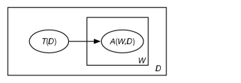
Figure 17.9 shows a plate representation of a model where a document, represented as a set of words, has a single topic. In this model:
-
•
is the set of all documents
-
•
is the set of all words
-
•
is a parametrized random variable such that Boolean is true if word appears in document
-
•
is a parametrized random variable such that , with domain the set of all topics, is the topic of document .
In this model, the topic for a document is connected to all words. There is no aggregation, as there are no arcs out of a plate. The documents are independent of each other.
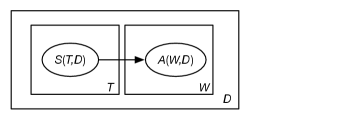
Figure 17.10 shows a plate representation of a model where a document, represented as a set of words, can have multiple topics. Instead of having a random variable with domain the set of all topics – implying a document can only have a single topic – there is a Boolean random variable for each topic and document:
-
•
is the set of all documents
-
•
is the set of all words
-
•
is the set of all topics (with a slight abuse of notation from the previous model)
-
•
Boolean is true if word appears in document
-
•
Boolean is true if topic is a subject of document .
In this model, all topics for a document are connected to all words. The documents are independent of each other. The grounding for a single document is show in Figure 9.29. Because there is an arc out of a plate, this model requires a form of aggregation. Noisy-or was used in Google’s Rephil; see Example 9.38.
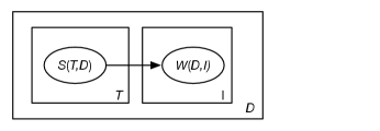
Figure 17.11 is like the previous case, but with a bag-of-words (unigram) model of each document. In this model
-
•
is the set of all documents
-
•
is the set of indexes of words in the document; ranges from to the number of words in the document
-
•
is the set of all topics
-
•
is the ’th word in document ; the domain of is the set of all words.
-
•
is true if topic is a subject of document ; is Boolean.
Example 17.9.
Consider a document, , that just consists of the words “the cat sat on the mat”, and suppose there are three topics, animals, football, and AI.
In a set-of-words model, there is a Boolean random variable for each word. To condition on this document, and are observed to be true. is observed to be false, because the word “neural” does not appear in the document. Similarly for the other words.
In a bag-of-words model, there is a random variable for each position in the document, with domain the set of all words. In this model, the observation about document is , , etc., and where is a value representing the end of the document.
In Figure 17.9 there is a single topic for each document. This is represented by the random variable with domain .
In the other two models, with document possibly containing multiple topics, there is a Boolean random variable for each topic. In this case there are three random variables, including that is true when animals is a topic of document , and that is true when football is a topic of document .
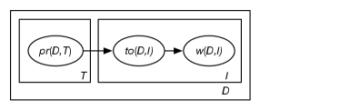
Figure 17.12 shows a model called latent Dirichlet allocation (LDA), with the following meaning:
-
•
is the document and is the index of a word in the document.
-
•
is the topic.
-
•
is the th word in document . The domain of is the set of all words; thus, this is a bag-of-words model.
-
•
is the topic of the th word of document . The domain of is the set of all topics. gives the word distribution over each topic.
-
•
represents the proportion of document that is about topic . The domain of is the reals. If is positive (pseudo)counts, this is a Dirichlet distribution, with
Alternatively, could be represented as a softmax, with
which is similar to an attention mechanism, where each word pays attention to the topics.
To go beyond set-of-words and bag-of-words, for example, to model the sequence of words an -gram, more structure is needed than is specified by a plate model. In particular, these require the ability to refer to the sequence previous words, which can be represented using structure in the logical variables (plates), such as can be provided by function symbols in logic.
17.3.4 Some Specific Representations
Any of the representations of belief networks can be used for representing relational probabilistic models. However, because plates correspond to logical variables, representations defined in terms of first-order logic most naturally represent these models. The models can also provide structure in the logical variables. In the neural network literature, plate models are referred to as convolutional models, due to the parameter sharing, which also corresponds to universal quantification in logic.
The representations mainly differ in the way they handle aggregation, and whether latent features are random variables or tunable weighted formulas (as in neural networks).
Some notable representations include the following.
Probabilistic Logic Programs
In a probabilistic logic program, the model is described in terms of a logic program with parametrized noise variables. Plates correspond to logical variables.
Example 17.10.
To represent the domain of Figure 17.7, as described in Example 17.8:
Each instance of and are parameterized noise variables. is the probability that was shot even if no one shot them. is the probability that would be shot if shot . These two rules implement a noisy-or over the instances of for each . The parametrized random variable can be represented using rules such as:
is the probability that would shoot if they had a motive, gun, and opportunity. Other rules could cover cases such as where doesn’t have motive.
Probabilistic logic programs go beyond the plate model, as they can handle recursion, which gives loops in the lifted model.
Weighted First-Order Logic Formulas
An alternative is to use weighted formulas, where the formulas contain logical variables, corresponding to the plates. The formulas can either define a directed model, called relational logistic regression, or an undirected, called a Markov logic network (MLN).
Example 17.11.
The domain of Figure 17.7 can be represented using the weighted formulas
where , , and are weights that are shared by all ground instances of the corresponding formula. Note that the last weighted formula has the same form as an implication with conjunctions in the body; it is true for all cases except for exceptions to the rule.
Inference in Markov logic networks and in models with relational logistic regression require marginalizing unobserved variables in the grounding. Probabilistic soft logic has weighted logical formulas like Markov logic networks, but the latent variables are represented like latent features in neural networks. This means that inference is much faster, as marginalization is avoided, and learning can use standard gradient descent methods. It means that the latent variables cannot be interpreted as random variables, which may make interpretation more difficult.
Directed models, such as probabilistic logic programs, have the advantages of being able to prune irrelevant variables in the grounding – in cases such as truth discovery, most are pruned – and being able to be learned modularly. One problem with the grounding being a belief network is the need for it to be acyclic, for example might depend on , and making the grounding acyclic entails arbitrary orderings. Relational dependency networks are directed models that allow cycles. The probabilities in the model define the transitions in a Markov chain. The distribution defined by the model is the stationary distribution of the induced Markov chain.
Graph Neural Networks
Graph neural networks are neural networks that act on graph data. Each node has an embedding that is inferred from parametrized linear functions and activation functions of the node’s neighbors, and their neighbors, to some depth.
A relational graph convolutional network (R-GCN) is used to learn embeddings for knowledge graphs, where nodes are entities and arcs are labelled with relations. The properties for entity in the knowledge graph are used to give an embedding , similar to the encoder used for word embeddings. These embeddings provide inputs to the neural network. There are multiple layers, with shared parameters, that follow the graph structure to give an output embedding for each entity.
The output embedding for an entity can be used to predict properties of the entity, or can be used in models such as polyadic decomposition to predict arcs. It is called convolutional because, like other relational models, the same learnable parameters for the layers are used for each entity. These layers provide separate embeddings for each entity based on the properties of the entity and its local neighborhood.
The layers are defined as follows. The embedding of layer for entity is the vector defined in terms of the embeddings of and its neighbors in the knowledge graph in the previous layer:
where is an activation function, such as ReLU, defined by . is the set of all relations and is the set of triples in the knowledge graph. is the embedding for entity from layer . is a matrix for relation for layer , which is multiplied by the vector for each neighbor . is a matrix defining how the embedding for entity in layer affects the same entity in the next layer. is a normalization constant, such as , which gives an average for each relation. The base case is , which doesn’t use any neighborhood information.
This model uses separate parameters for each relation, which can result in overfitting for relations with few instances. To help solve this, the relation matrices, , can be represented as a linear combination of learned basis matrices which are shared among the relations; the weights in the linear combination depend on the relation.
Whereas the embedding-based models of Section 17.2.2 did not work well for reified entities, because reified entities had very few instances, the use of two or more layers in relational graph convolutional network allows a node to depend on the neighbors of neighbors.
The depth of the network is directly related to the size of the neighborhood of a node used. A network of size uses paths of length from each node.
The methods based on lifted graphical models work the same whether the intermediate variables are observed or not. For example, in the shooting example, can depend on other parametrized random variables, such as whether someone hired to shoot (see Example 17.5), in which case needs to be marginalized out. However, graph neural networks treat relations specified in the knowledge graph differently from inferred relations, and thus need to learn the model as a function of the specified relations. This lack of modularity makes them less flexible.
Artificial Intelligence: Foundations of Computational Agents, Poole
& Mackworth
Copyright © 2023, David L. Poole and Alan K. Mackworth. 
This work is licensed under a Creative Commons Attribution-NonCommercial-NoDerivatives 4.0 International License.