Artificial
Intelligence 3E
foundations of computational agents
17.2 Embedding-Based models
17.2.1 Learning a Binary Relation
Suppose you are given a database of a binary relation where both arguments are entities, and the aim is to predict whether other tuples are true. The machine learning methods of Chapters 7 and 8 are not directly applicable as the entities are represented using meaningless names (identifiers). An algorithm that does this is defined below, for the case where there are no other relations defined, but where there can also be a numeric prediction for the pair. This is explained using a particular example of predicting a user’s ratings for an item such as a movie.
In a recommender system, users are given personalized recommendations of items they may like. One technique for recommender systems is to predict the rating of a user on an item from the ratings of similar users or similar items, by what is called collaborative filtering.
Example 17.1.
MovieLens (https://movielens.org/) is a movie recommendation system that acquires movie ratings from users. The rating is from 1 to 5 stars, where 5 stars is better. The first few tuples of one dataset are shown in Table 17.1,
| User | Item | Rating | Timestamp |
|---|---|---|---|
| 196 | 242 | 3 | 881250949 |
| 186 | 302 | 3 | 891717742 |
| 22 | 377 | 1 | 878887116 |
| 244 | 51 | 2 | 880606923 |
| 253 | 465 | 5 | 891628467 |
| … | … | … | … |
where each user is given a unique number, each item (movie) is given a unique number, and the timestamp is the Unix standard of seconds since 1970-01-01 UTC. Such data can be used in a recommendation system to make predictions of other movies a user might like.
One way for a recommender system to personalize recommendations is to present the user with the top-n items, where is a positive integer, say 10. This can be done by first estimating the rating of each item for a user and then presenting the items with the highest predicted rating. This is not a good solution in general, as all of the top items might be very similar. The system should also take diversity into account when choosing the set of items.
In the example above, the items were movies, but they could also be consumer goods, restaurants, holidays, or other items.
Netflix Prize
There was a considerable amount of research on collaborative filtering with the Netflix Prize to award $1,000,000 to the team that could improve the prediction accuracy of Netflix’s proprietary system, measured in terms of sum-of-squares, by 10%. Each rating gives a user, a movie, a rating from 1 to 5 stars, and a date and time the rating was made. The dataset consisted of approximately 100 million ratings from 480,189 anonymized users on 17,770 movies that was collected over a 7-year period. The prize was won in 2009 by a team that averaged over a collection of hundreds of predictors, some of which were quite sophisticated. After 3 years of research, the winning team beat another team by just 20 minutes to win the prize. They both had solutions which had essentially the same error, which was just under the threshold to win. Interestingly, an average of the two solutions was better than either alone.
The algorithm presented here is the basic algorithm that gave the most improvement.
The Netflix dataset is no longer available because of privacy concerns. Although users were only identified by a number, there was enough information, if combined with other information, to potentially identify some of the users.
Suppose is a dataset of triples, where means user gave item a rating of (ignoring the timestamp). Let be the predicted rating of user on item . The aim is to optimize the sum-of-squares error
As with most machine learning, the aim is to optimize for the test examples, not for the training examples.
Following is a sequence of increasingly sophisticated models for , the prediction of the rating of a user for an item. Each model adds more terms to the model, in a similar way to how features are added in boosting and residuals in deep learning.
- Make a single prediction
-
The simplest case is to predict the same rating for all users and items: , where is the mean rating. Recall that when predicting the same value for every instance, predicting the mean minimizes the sum-of-squares error.
- Add user and item biases
-
Some users might give higher ratings than other users, and some movies may have higher ratings than other movies. You can take this into account using
where user has bias and item has bias . The parameters and are chosen to minimize the sum-of-squares error. If there are users and items, there are parameters to tune (assuming is fixed). Finding the best parameters is an optimization problem that can be done with a method like gradient descent, as was used for the linear learner.
One might think that should be directly related to the average rating for user and should be directly related to the average rating for item . However, it is possible that even if all of the ratings for user were above the mean . This can occur if user only rated popular items and rated them lower than other people.
Optimizing the and parameters can help get better estimates of the ratings, but it does not help in personalizing the recommendations, because the movies are still ordered the same for every user.
- Add a latent property
-
You could hypothesize that there is an underlying property of each user and each movie that enables more accurate predictions, such as the age of each user, and the age-appeal of each movie. A real-valued latent property or hidden property for each entity can be tuned to fit the data.
Suppose the latent property for user has a value , and the latent property for item has value . The product of these is used to offset the rating of that item for that user:
If and are both positive or both negative, the property will increase the prediction. If one of or is negative and the other is positive, the property will decrease the prediction.
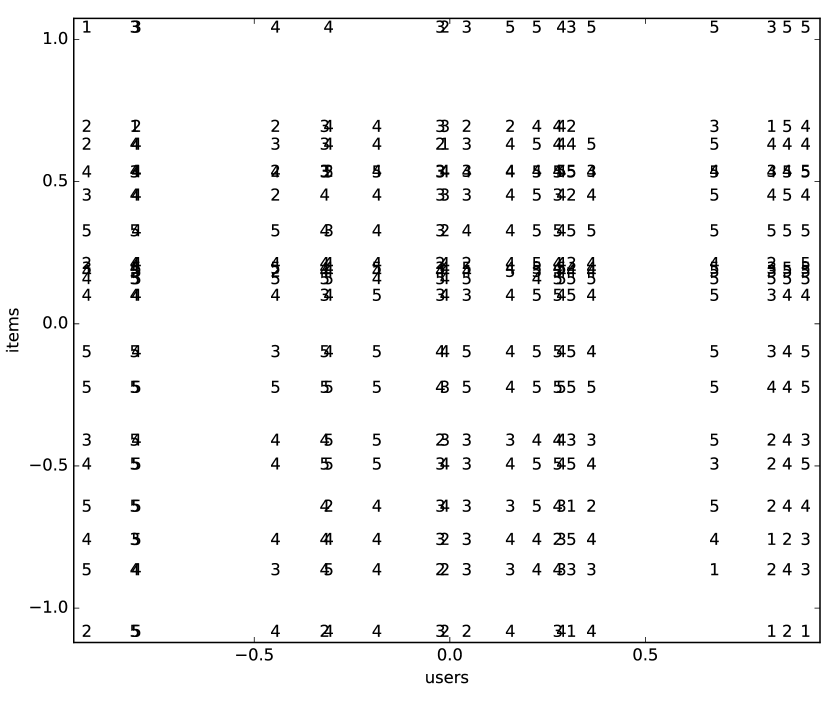
Figure 17.1: Movie ratings as a function of a single latent property; see Example 17.2 Example 17.2.
Figure 17.1 shows a plot of the ratings as a function of a single latent property. This uses the subset of the MovieLens 100k dataset, containing the 20 movies that had the most ratings, and the 20 users who had the most ratings for these movies. It was trained for 1000 iterations of gradient descent, with a single latent property.
On the -axis are the users, ordered by their value, , on the property. On the -axis are the movies, ordered by their value, on the property. Each rating is then plotted against the user and the movie, so that triple is depicted by plotting at the position . Thus each vertical column of numbers corresponds to a user, and each horizontal row of numbers is a movie. The columns overlap if two users have very similar values on the property. The rows overlap for movies that have very similar values on the property. The users and the movies where the property values are close to zero are not affected by this property, as the prediction uses the product of values of the properties.
In general, high ratings are in the top-right and the bottom-left, as these are the ratings that are positive in the product, and low ratings in the top-left and bottom-right, as their product is negative. Note that what is high and low is relative to the user and movie biases; what is high for one movie may be different from what is high for another movie.
- Add latent properties
-
Instead of using just one property, consider using latent properties for each user and item. There is a value (using Python notation for matrices) for each user and property . The vector of length is called the user embedding for user , analogous to the word embeddings used in deep learning. Similarly, there is a value for every item and property , where is the item embedding for item . The contributions of the separate properties are added. This gives the prediction
This is often called a matrix factorization method as the summation corresponds to matrix multiplication of and the transpose – flipping the arguments – of .
- Regularize
-
To avoid overfitting, a regularization term can be added to prevent the parameters from growing too much and overfitting the given data. Here an regularizer for each of the parameters is added to the optimization. The goal is to choose the parameters to
(17.1) where is a regularization parameter, which can be tuned by cross validation.
The parameters , , , and can be optimized using stochastic gradient descent, as shown in Figure 17.2. The parameters there are adjusted in each iteration, but regularized after going through the dataset, which might not be the best choice; see Exercise 17.3. Note that the elements of and need to be initialized randomly (and not to the same value) to force each property to be different.
To understand what is being learned, consider the following thought experiment:
Example 17.3.
In the rating running example, suppose there is a genre of movies that some people really like and others hate. Suppose property has 1 for movies of that genre, and 0 for other movies. Users who like that genre more than would be expected from other properties have a high value for property , those that dislike it more have a negative value, and others have values close to zero. This can be seen as a soft clustering – as in expectation maximization (EM) – for users into the categories of likes, dislikes, and indifferent. Suppose now that the user property is fixed to these values, but the corresponding property for the movie is learned, so it might not exactly correspond to the genre. The movies that have a high value for the property are the movies that are liked by the people who like the genre and disliked by those who hate the genre. Thus it learns which movies those people like or dislike. Again it is providing a soft clustering of movies. With multiple latent properties, it can find multiple soft clusterings, with the values added together in a similar way to boosting and residuals in deep learning.
The alternating least squares algorithm acts like the above description, alternating fixing user or item properties and optimizing the other, but starting with random assignments. Optimizing Equation 17.1 with user or item parameters fixed gives a linear regression on the other parameters. The adjustments in Figure 17.2 are more fine grained, but the results are similar.
This algorithm can be evaluated by how well it predicts future ratings by training it with the data up to a certain time, and testing it on future data.
The algorithm can be modified to take into account observed attributes of items and users by fixing some of the properties. For example, the Movielens dataset includes 19 genres, which can be represented using 19 of the embedding positions, one position for each genre (forming a one-hot encoding for part of the embedding space). If position represents a particular genre, a movie has 1 at position if the movie has the corresponding genre and 0 otherwise. Each user has a learnable parameter at position to indicate whether the genre is positive or negative for that user, as in Example 17.3. Different positions are used for user properties. Using explicit properties is useful when users or items have few ratings from which to learn, or for the cold-start problem, which is how to make recommendations about new items or for new users; predictions can be made just on the observed properties, without any ratings needed.
This algorithm ignores the timestamp, but using the timestamp may help as users’ preferences may change and items may come in and out of fashion. The dynamics of preferences becomes important when predicting future ratings – which is usually what is wanted – but there is usually very little data to learn the dynamics for each user.
The above was for regression, predicting the numerical rating of an item for a user. For Boolean classification, for example, whether the rating is greater than 3, the sigmoid of a linear function provides a probabilistic prediction. When trained to optimize binary log loss, the algorithm can remain unchanged, except for an added sigmoid in the definition of on line 11 of Figure 17.2.
The Boolean function of whether a rating is greater than 3 is atypical because both positive and negative examples are provided. Most relations do not contain negative examples. For some, the closed-world assumption – everything not stated is false – may be appropriate, but then there is nothing to learn. For relations where only positive examples are provided, for example predicting , which is true when a rating is provided, the above algorithm will conclude that everything is true, as that prediction minimizes Equation 17.1. The mean value ( in Figure 17.2) is not defined. To handle this case, either can be treated as a parameter which must be regularized, or negative examples need to be provided. The ratio of positive to negative examples and the regularization parameter both provide a prior assumption of the probability, which is not something that can be estimated from the data. Because the algorithm can handle noise, it is reasonable to just choose random cases as negative examples, even though they could be positive. The absence of negative examples also makes evaluation challenging and is one reason why relational prediction methods are often judged using ranking, such as predicting the top-n items for each user.
When used for recommendations, it might be better to take the diversity of the recommendations into account and recommend very different items than to recommend similar items. Thus, while predicting the ratings is useful, it does not lead directly to useful recommendations.
17.2.2 Learning Knowledge Graphs
Suppose the aim is to learn the triples of a knowledge graph. Consider predicting the truth of the triple , where is the subject, is the relation (verb), and the object of the triple. A straightforward extension to matrix factorization to predict triples is the polyadic decomposition, which decomposes a tensor into matrices. It can be used to predict the probability of a triple – an element of a three-dimensional tensor – as
using the tunable parameters
-
•
a global bias
-
•
two biases for each entity , namely , used when is in the first position, and , used when is in the third position
-
•
a bias for each relation , given by
-
•
a matrix , indexed by entities and properties, so that is the vector of length , called the subject embedding for , used when appears as the first item of a triple, and a matrix , providing the object embedding for each entity when it appears as the third item of a triple
-
•
a matrix , indexed by relations and properties, where is the relation embedding for relation .
All of the embeddings , , and are the same length.
Training this model on a dataset of triples, minimizing categorical log loss with L2 regularization, is like the algorithm of Figure 17.2, but with a different predictor and more parameters to tune and regularize. With only a knowledge graph of triples with no negative examples, as with the binary case above, without regularizing , all triples being true minimizes the error. Either negative examples need to be added or regularization of is required. The ratio of positive to negative examples, and the regularization of , convey prior information about the proportion of tuples expected to be true, which cannot be obtained from a dataset of only positive triples.
The polyadic decomposition, however, does not work well because the subject and object embeddings are independent of each other.
Example 17.4.
Suppose user likes movies directed by a particular person , and the knowledge is represented as and . Whether someone likes a movie only depends on the object embedding of the movie, but the directorship depends only on the subject embedding of the movie. As these embeddings do not interact, there is no way for the above embedding model to represent the interdependence. A solution to this is to also represent the inverse of the relations where and .
The polyadic decomposition with inverses has embeddings for each relation and its inverse , where , to make the prediction that is the average of the prediction from the two ways of representing the same tuple:
where is the prediction from the polyadic decomposition. This allows the interdependence of the subject and object embeddings, which can solve the problem of Example 17.4.
The polyadic decomposition with inverses is fully expressive, meaning it can approximate any relation with a log loss less than and , even if all embeddings are restricted to be non-negative, and the value of all embedding values is bounded by a constant (which may depend on ). This means that it can memorize any relation, which is the best it can do in general; see the no-free-lunch theorem. It also means that there are no inherent restrictions on what can be represented. If the same embedding is used for the subject and the object, only symmetric relations can be represented or approximated.
Example 17.3 explains how the user and items embedding used in prediction can be used to understand what is being learned. That explanation holds for a relation, for each embedding position where the relation has a non-zero value. In particular, for the case where all embeddings are non-negative:
-
•
For the subject embedding, each embedding position is a soft clustering of entities. Those entities in the cluster have a large value for that position, where large is relative to the other values. Similarly, for the object embedding.
-
•
For each position, the product of the subject, relation, and object embeddings is only large if all three are large. When the relation embedding is large at a position, the entities in the subject clustering for that position are related to the entities in the corresponding object clustering.
-
•
The addition () provides for multiple clusterings to be added together.
In the general case, when an even number of the values being multiplied are negative, the result is positive and it acts like the above. When an odd number of the values is negative (one or three of the subject, relation, and object is negative), the product is negative and this position can act like exceptions.
This method – and related methods – is clustering entities in various ways to provide the best predictions. What is learned is not general knowledge that can be applied to other populations. If the goal is to model a single population, for example in a social network, that might be adequate. However, if the aim is to learn knowledge that can be applied to new populations, this method does not work.
Decomposing a relation into matrices does not work well for relations with multiple arguments. If the relation is converted to triples using reification, the introduced entity has very few instances – the number of arguments to the relation – which makes learning challenging. If the polyadic deposition is used directly, the problem of independent positions – which motivated the inverses above – occurs for every pair of positions. Modeling the interaction between every pair of argument predictions leads to overfitting.
Embedding-based models that decompose a relation do not work for predicting properties with a fixed range, such as the age of users, because they rely on a lower-dimensional representation and there isn’t one for properties. The vector for a user can be used to memorize the age in one or more of the embedding positions, which means it does not generalize.
Artificial Intelligence: Foundations of Computational Agents, Poole
& Mackworth
Copyright © 2023, David L. Poole and Alan K. Mackworth. 
This work is licensed under a Creative Commons Attribution-NonCommercial-NoDerivatives 4.0 International License.