Artificial
Intelligence 3E
foundations of computational agents
12.1 Preferences and Utility
What an agent decides to do should depend on its preferences. This section specifies some intuitive properties of preferences and gives some consequences of those properties. The properties are axioms of rationality. You should consider whether each axiom is reasonable for a rational agent to follow; if you accept them all as reasonable, you should accept their consequences. If you do not accept the consequences, you need to give up one or more of the axioms.
12.1.1 Axioms for Rationality
An agent chooses actions based on their outcomes. Outcomes are whatever the agent has preferences over. If an agent does not prefer any outcome to any other outcome, it does not matter what the agent does. Initially, let’s consider outcomes without considering the associated actions. Assume there are only a finite number of outcomes.
Let’s define a preference relation over outcomes. Suppose and are outcomes. Outcome is weakly preferred to outcome , written , if outcome is at least as desirable as outcome .
We write to mean the negation of , that is, is not weakly preferred to outcome .
Define to mean and . That is, means outcomes and are equally preferred. In this case, we say that the agent is indifferent between and .
Define to mean and . That is, the agent weakly prefers outcome to outcome , but does not weakly prefer to , and is not indifferent between them. In this case, we say that outcome is strictly preferred to outcome .
Typically, an agent does not know the outcome of its actions. A lottery is defined to be a finite distribution over outcomes, written
where each is an outcome and each is a non-negative real number such that . The lottery specifies that outcome occurs with probability . In all that follows, assume that outcomes may include lotteries. This includes lotteries where the outcomes are also lotteries (called lotteries over lotteries).
Axiom 12.1.
(Completeness) An agent has preferences between all pairs of outcomes:
The rationale for this axiom is that an agent must act; if the actions available to it have outcomes and then, by acting, it is explicitly or implicitly preferring one outcome over the other.
Axiom 12.2.
(Transitivity) Preferences are transitive:
To see why this is reasonable, suppose it is false, in which case and and . Because is strictly preferred to , the agent should be prepared to pay some amount to get from to . Suppose the agent has outcome ; then is at least as good so the agent would just as soon have . is at least as good as , so the agent would just as soon have as . Once the agent has , it is again prepared to pay to get to . It has gone through a cycle of preferences and paid money to end up where it is. This cycle that involves paying money to go through it is known as a money pump because, by going through the loop enough times, the amount of money that an agent must pay can exceed any finite amount. It seems reasonable to claim that being prepared to pay money to cycle through a set of outcomes is irrational; hence, a rational agent should have transitive preferences.
It follows from the transitivity and completeness axioms that transitivity holds for mixes of and , so that , then and if one or both of the preferences in the premise of the transitivity axiom is strict, then the conclusion is strict. Thus, , then . See Exercise 12.1.
Axiom 12.3.
(Monotonicity) An agent prefers a larger chance of getting a better outcome than a smaller chance of getting the better outcome, other things being equal. That is, if and , then
Note that, in this axiom, between outcomes represents the agent’s preference, whereas between and represents the familiar comparison between numbers.
The following axiom specifies that lotteries over lotteries only depend on the outcomes and probabilities.
Axiom 12.4.
(Decomposability) (“no fun in gambling”) An agent is indifferent between lotteries that have the same probabilities over the same outcomes, even if one or both is a lottery over lotteries. For example:
Also for any outcomes and .
This axiom specifies that it is only the outcomes and their probabilities that define a lottery. If an agent had a preference for gambling, that would be part of the outcome space.
These four axioms imply some structure on the preference between outcomes and lotteries. Suppose that and . Consider whether the agent would prefer
-
•
or
-
•
the lottery
for different values of . When , the agent prefers the lottery (because, by decomposability, the lottery is equivalent to and ). When , the agent prefers (because the lottery is equivalent to and ). At some stage, as is varied, the agent’s preferences flip between preferring and preferring the lottery.
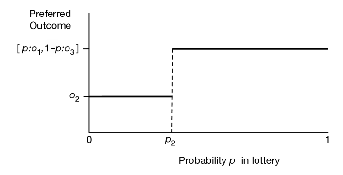
Figure 12.1 shows how the preferences must flip as is varied. On the -axis is and the -axis shows which of or the lottery is preferred. The following proposition formalizes this intuition.
Proposition 12.1.
If an agent’s preferences are complete, transitive, and follow the monotonicity axiom, and if and , there exists a number such that and
-
•
for all , the agent prefers to the lottery (i.e., ) and
-
•
for all , the agent prefers the lottery (i.e., ).
Proof.
By monotonicity and transitivity, if for any , then, for all , . Similarly, if for any , then, for all , .
By completeness, for each value of , either , , or . If there is some such that , then the theorem holds. Otherwise, a preference for either or the lottery with parameter implies preferences for either all values greater than or for all values less than . By repeatedly subdividing the region that we do not know the preferences for, we will approach, in the limit, a value filling the criteria for . ∎
The preceding proposition does not specify what the preference of the agent is at the point . The following axiom specifies that the agent is indifferent at this point.
Axiom 12.5.
(Continuity) Suppose and , then there exists a such that
The next axiom specifies that replacing an outcome in a lottery with an outcome that is not worse, cannot make the lottery worse.
Axiom 12.6.
(Substitutability) If then the agent weakly prefers lotteries that contain instead of , everything else being equal. That is, for any number and outcome :
A direct corollary of this is that outcomes to which the agent is indifferent can be substituted for one another, without changing the preferences.
Proposition 12.2.
If an agent obeys the substitutability axiom and , then the agent is indifferent between lotteries that only differ by and . That is, for any number and outcome , the following indifference relation holds:
This follows because is equivalent to and , and we can use substitutability for both cases.
An agent is defined to be rational if it obeys the completeness, transitivity, monotonicity, decomposability, continuity, and substitutability axioms.
It is up to you to determine if this technical definition of rationality matches your intuitive notion of rationality. In the rest of this section, we show more consequences of this definition.
Although preferences may seem to be complicated, the following theorem shows that a rational agent’s value for an outcome can be measured by a real number. Those value measurements can be combined with probabilities so that preferences with uncertainty can be compared using expectation. This is surprising for two reasons:
-
•
It may seem that preferences are too multifaceted to be modeled by a single number. For example, although one may try to measure preferences in terms of dollars, not everything is for sale or easily converted into dollars and cents.
-
•
One might not expect that values could be combined with probabilities. An agent that is indifferent between the money and the lottery for all monetary values and and for all is known as an expected monetary value (EMV) agent. Most people are not EMV agents, because they have, for example, a strict preference between $1,000,000 and the lottery . (Think about whether you would prefer a million dollars or a coin toss where you would get nothing if the coin lands heads or two million if the coin lands tails.) Money cannot be simply combined with probabilities, so it may be surprising that there is a value that can be.
Proposition 12.3.
If an agent is rational, then for every outcome there is a real number , called the utility of , such that
-
•
if and only if and
-
•
utilities are linear with probabilities
Proof.
If the agent has no strict preferences (i.e., the agent is indifferent between all outcomes), then define for all outcomes .
Otherwise, choose the best outcome, , and the worst outcome, , and define, for any outcome , the utility of to be the value such that
The first part of the proposition follows from substitutability and monotonicity.
To prove the second part, any lottery can be reduced to a single lottery between and by replacing each by its equivalent lottery between and , and using decomposability to put it in the form , with equal to . The details are left as an exercise. ∎
Thus, an ordinal preference that follows the axioms is a cardinal preference where utility defines the values to be compared.
In this proof the utilities are all in the range , but any linear scaling gives the same result. Sometimes is a good scale to distinguish it from probabilities, and sometimes negative numbers are useful to use when the outcomes have costs. In general, a program should accept any scale that is intuitive to the user.
A linear relationship does not usually exist between money and utility, even when the outcomes have a monetary value. People often are risk averse when it comes to money: they would rather have in their hand than some randomized setup where they expect to receive but could possibly receive more or less.
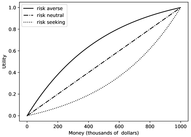
Example 12.1.
Figure 12.2 shows a possible money–utility relationship for three agents. The topmost line represents an agent that is risk averse, with a concave utility function. The agent with a straight-line plot is risk neutral. The lowest line represents an agent with a convex utility function that is risk seeking.
The risk-averse agent in Figure 12.2 would rather have $300,000 than a 50% chance of getting either nothing or $1,000,000, but would prefer the gamble on the million dollars to $275,000. This can be seen by checking the value for . They would also require more than a 73% chance of winning a million dollars to prefer this gamble to half a million dollars.
For the risk-averse agent, . Thus, given this utility function, the risk-averse agent would be willing to pay $1000 to eliminate a chance of losing all of their money. This is why insurance companies exist. By paying the insurance company, say, $600, the risk-averse agent can change the lottery that is worth $999,000 to them into one worth $1,000,000 and the insurance companies expect to pay out, on average, about $300, and so expect to make $300. The insurance company can get its expected value by insuring enough houses. It is good for both parties.
Rationality does not impose any conditions on what the utility function looks like.
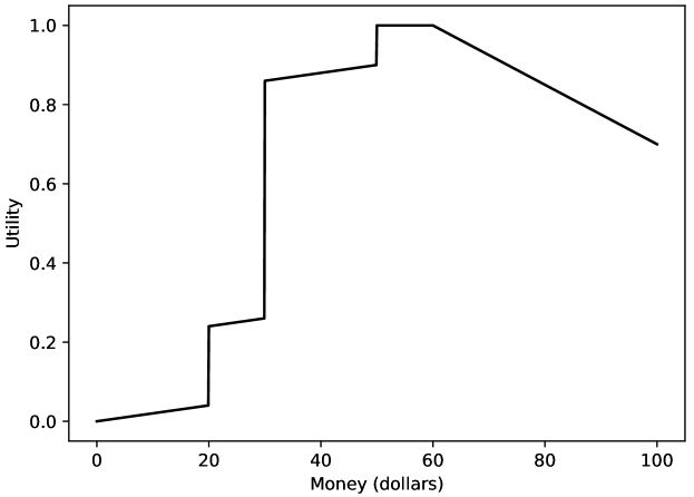
Example 12.2.
Figure 12.3 shows a possible money–utility relationship for Chris who really wants a toy worth , but would also like one worth , and would like both even better. Apart from these, money does not matter much to Chris. Chris is prepared to take risks. For example, if Chris had , Chris would be very happy to bet against a single dollar of another agent on a fair bet, such as a coin toss. This is reasonable because that $9 is not much use to Chris, but the extra dollar would enable Chris to buy the toy. Chris does not want more than , because then Chris will worry about it being lost or stolen.
Challenges to Expected Utility
There have been a number of challenges to the theory of expected utility. The Allais Paradox, presented in 1953 [Allais and Hagen, 1979], is as follows. Which would you prefer of the following two alternatives?
-
A:
$1m – one million dollars
-
B:
lottery 5m, 1m, .
Similarly, what would you choose between the following two alternatives?
-
C:
lottery m,
-
D:
lottery m, .
It turns out that many people prefer to , and prefer to . This choice is inconsistent with the axioms of rationality. To see why, both choices can be put in the same form:
-
A,C:
lottery m,
-
B,D:
lottery m, , .
In and , is a million dollars. In and , is zero dollars. Concentrating just on the parts of the alternatives that are different seems intuitive, but people seem to have a preference for certainty.
Tversky and Kahneman [1974], in a series of human experiments, showed how people systematically deviate from utility theory. One such deviation is the framing effect of a problem’s presentation. Consider the following.
-
•
A disease is expected to kill 600 people. Two alternative programs have been proposed:
-
Program A:
200 people will be saved
-
Program B:
with probability , 600 people will be saved, and with probability , no one will be saved.
Which program would you favor?
-
Program A:
-
•
A disease is expected to kill 600 people. Two alternative programs have been proposed:
-
Program C:
400 people will die
-
Program D:
with probability , no one will die, and with probability , 600 will die.
Which program would you favor?
-
Program C:
Tversky and Kahneman showed that 72% of people in their experiments chose program A over program B, and 22% chose program C over program D. However, these are exactly the same choice, just described in a different way.
Prospect theory, developed by Kahneman and Tversky, is an alternative to expected utility that better fits human behavior.
12.1.2 Factored Utility
Utility for an agent is a function of outcomes or states. Representing utilities in terms of features or variables typically results in more compact representations that are easier to reason with and more natural to acquire.
Suppose each outcome can be described in terms of features . An additive utility is one that can be decomposed into a sum of terms:
Such a decomposition is making the assumption of additive independence.
When this can be done, it greatly simplifies preference elicitation – the problem of acquiring preferences from the user. This decomposition is not unique, because adding a constant to one of the terms and subtracting it from another gives the same utility. A canonical representation for additive utility has a unique decomposition. Canonical forms are easier to acquire as each number can be acquired without considering the other numbers. To put additive utility into canonical form, for each feature , define a local utility function that has a value of 0 for the value of in the worst outcome and 1 for the value of in the best outcome, and a non-negative real weight, . The weights should sum to 1. The utility as a function of the variables is
To elicit such a utility function requires eliciting each local utility function and assessing the weights. Each feature, if it is relevant, must have a best value for an agent and a worst value for the agent. Assessing the local functions and weights can be done as follows. Consider just ; the other features then can be treated analogously. For feature , values and for , and fixed values for :
| (12.1) |
The weight can be derived when is the best outcome and is the worst outcome (because then ). The values of for the other values in the domain of can be computed using Equation 12.1, making the worst outcome (as then ).
Assuming additive independence entails making a strong independence assumption. In particular, in Equation 12.1, the difference in utilities must be the same for all values for .
Additive independence is often not a good assumption. Consider binary features and , with domains and .
-
•
Two values of and are complements if having both is better than the sum of having the two separately. More formally, values and are complements if getting one when the agent has the other is more valuable than when the agent does not have the other:
-
•
Two values are substitutes if having both is not worth as much as the sum of having each one. More formally, values and are substitutes if getting one when the agent has the other is less valuable than getting one when the agent does not have the other:
Example 12.3.
For a purchasing agent in the travel domain, consider the utility function for having a plane booking for a particular day and a hotel booking for the same day:
| Plane | Hotel | Utility |
|---|---|---|
| 100 | ||
| 0 | ||
| 10 | ||
| 20 |
Thus
Thus, a plane booking and a hotel booking are complements: one without the other does not give a good outcome.
If the person taking the holiday would enjoy one outing, but not two, on the same day, the two outings on the same day would be substitutes.
Additive utility assumes there are no substitutes or complements. When there is interaction, we require a more sophisticated model, such as a generalized additive independence model, which represents utility as a sum of terms, where each term can be a factor over multiple variables. Elicitation of the generalized additive independence model is much more involved than eliciting an additive model, because a variable can appear in many factors.
For Boolean features, it is possible to represent arbitrary utility using the analogy to the canonical representation for probability. This extends the additive utility to allow weights for the conjunctions of atoms (which corresponds to the product when true is 1 and false is 0), including a bias term. Complements have a positive weight for the conjunction, and substitutes have a negative weight for the conjunction.
Example 12.4.
Consider Example 12.3. The utility for a plane and a hotel for the same day, as shown in the table, can be represented using
where , , , .
For the two trips in Example 12.3, where the person does not want both, the weight for the product term would be negative.
It is common to start with representing just the simpler interactions, such as only representing the weights of single atoms and some pairwise products, and only introducing products of more atoms when necessary. If all conjunctions were included, there would be weights for propositions, which is the same as a table of all combinations of truth values. The canonical representation is useful when many of the weights are zero, and so don’t need to be represented at all.
12.1.3 Prospect Theory
Utility theory is a normative theory of rational agents that is justified by a set of axioms. Prospect theory is a descriptive theory of people that seeks to describe how humans make decisions. A descriptive theory is evaluated by making observations of human behavior and by carrying out controlled psychology experiments.
Rather than having preferences over outcomes, prospect theory considers the context of the preferences. The idea that humans do not perceive absolute values, but values in context, is well established in psychology. Consider the Müller-Lyer illusion shown in Figure 12.4.
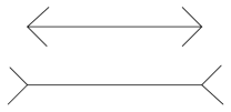
The horizontal lines are of equal length, but in the context of the other lines, they appear to be different. As another example, if you have one hand in cold water and one in hot water, and then put both into warm water, the warm water will feel very different to each hand. People’s preferences also depend on context. Prospect theory is based on the observation that it is not the outcomes that people have preferences over; what matters is how much the choice differs from the current situation.
The relationship between money and value that is predicted by prospect theory is shown in Figure 12.5.
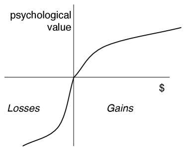
Rather than having the absolute wealth on the -axis, this graph shows the difference from the current wealth. The origin of the -axis is the current state of the person’s wealth. This position is called the reference point. Prospect theory predicts:
-
•
For gains, people are risk averse. This can be seen as the curve above the current wealth is concave.
-
•
For losses, people are risk seeking. This can be seen as the curve below the current wealth is convex.
-
•
Losses are approximately twice as bad as gains. The slope for losses is steeper than that for gains.
It is not just money that has such a relationship, but anything that has value. Prospect theory makes different predictions about how humans will act than does utility theory, as in the following examples from Kahneman [2011, pp. 275, 291].
Example 12.5.
Consider Anthony and Betty:
-
•
Anthony’s current wealth is $1 million.
-
•
Betty’s current wealth is $4 million.
They are both offered the choice between a gamble and a sure thing.
-
•
Gamble: equal chance to end up owning $1 million or $4 million.
-
•
Sure thing: own $2 million.
Utility theory predicts that, assuming they have the same utility curve, Anthony and Betty will make the same choice, as the outcomes are identical. Utility theory does not take into account the current wealth. Prospect theory makes different predictions for Anthony and Betty. Anthony is making a gain and so will be risk averse, and so will probably go with the sure thing. Betty is making a loss, and so will be risk seeking and go with the gamble. Anthony will be happy with the $2 million, and does not want to risk being unhappy. Betty will be unhappy with the $2 million, and has a chance to be happy if she takes the gamble.
Example 12.6.
Twins Andy and Bobbie, have identical tastes and identical starting jobs. There are two jobs that are identical, except that
-
•
job A gives a raise of $10,000
-
•
job B gives an extra day of vacation per month.
They are each indifferent to the outcomes and toss a coin. Andy takes job A, and Bobbie takes job B.
Now the company suggests they swap jobs with a $500 bonus.
Utility theory predicts that they will swap. They were indifferent and now can be $500 better off by swapping.
Prospect theory predicts they will not swap jobs. Given they have taken their jobs, they now have different reference points. Andy thinks about losing $10,000. Bobbie thinks about losing 12 days of holiday. The loss is much worse than the gain of the $500 plus the vacation or salary. They each prefer their own job.
Empirical evidence supports the hypothesis that prospect theory is better than utility theory in predicting human decisions. However, just because it better matches a human’s choices does not mean it is the best for an artificial agent. An artificial agent that must interact with humans should, however, take into account how humans reason. For the rest of this chapter we assume utility theory as the basis for an artificial agent’s decision making and planning.
Whose Values?
Any computer program or person who acts or gives advice is using some value system to judge what is important and what is not.
Alice went on “Would you please tell me, please, which way I ought to go from here?”
“That depends a good deal on where you want to get to,” said the Cat.
“I don’t much care where –” said Alice.
“Then it doesn’t matter which way you go,” said the Cat.
– Lewis Carroll (1832–1898)
Alice’s Adventures in Wonderland, 1865
We all, of course, want computers to work on our value system, but they cannot act according to everyone’s value system. When you build programs to work in a laboratory, this is not usually a problem. The program acts according to the goals and values of the program’s designer, who is also the program’s user. When there are multiple users of a system, you must be aware of whose value system is incorporated into a program. If a company sells a medical diagnostic program to a doctor, does the advice the program gives reflect the values of society, the company, the doctor, the patient, or whoever is paying (all of whom may have very different value systems)? Does it determine the doctor’s or the patient’s values?
For autonomous cars, do the actions reflect the utility of the owner or the utility of society? Consider the choice between injuring people walking across the road or injuring family members by swerving to miss the pedestrians. How do the values of the lives trade off for different values of and , and different chances of being injured or killed? Drivers who most want to protect their family would have different trade-offs than the pedestrians. This situation has been studied using trolley problems, where the trade-offs are made explicit and people give their moral opinions. See Section 2.4.
If you want to build a system that gives advice to someone, you should find out what is true as well as what their values are. For example, in a medical diagnostic system, the appropriate procedure depends not only on patients’ symptoms but also on their priorities. Are they prepared to put up with some pain in order to be more aware of their surroundings? Are they willing to put up with a lot of discomfort to live longer? What risks are they prepared to take? Always be suspicious of a program or person that tells you what to do if it does not ask you what you want to do! As builders of programs that do things or give advice, you should be aware of whose value systems are incorporated into the actions or advice. If people are affected, their preferences should be taken into account, or at least they should be aware of whose preferences are being used as a basis for decisions.
Artificial Intelligence: Foundations of Computational Agents, Poole
& Mackworth
Copyright © 2023, David L. Poole and Alan K. Mackworth. 
This work is licensed under a Creative Commons Attribution-NonCommercial-NoDerivatives 4.0 International License.