Third edition of Artificial Intelligence: foundations of computational agents, Cambridge University Press, 2023 is now available (including the full text).
10.3 Computing Strategies with Perfect Information
The equivalent to full observability with multiple agents is called perfect information. In perfect information games, agents act sequentially and, when an agent has to act, it gets to observe the state of the world before deciding what to do. Each agent acts to maximize its own utility.
A perfect information game can be represented as an extensive form game where the information sets all contain a single node. They can also be represented as a multiagent decision network where the decision nodes are totally ordered and, for each decision node, the parents of that decision node include the preceding decision node and all of their parents [i.e., they are no-forgetting decision networks].
Perfect information games are solvable in a manner similar to fully observable single-agent systems. We can either do it backward using dynamic programming or forward using search. The difference from the single-agent case is that the multiagent algorithm maintains a utility for each agent and, for each move, it selects an action that maximizes the utility of the agent making the move. The dynamic programming variant, called backward induction, essentially follows the definition of the utility of a node for each agent, but, at each node, the agent who controls the node gets to choose the action that maximizes its utility.
In the case where two agents are competing so that a positive reward for one is a negative reward for the other agent, we have a two-agent zero-sum game. The value of such a game can be characterized by a single number that one agent is trying to maximize and the other agent is trying to minimize. Having a single value for a two-agent zero-sum game leads to a minimax strategy. Each node is either a MAX node, if it is controlled by the agent trying to maximize, or is a MIN node if it is controlled by the agent trying to minimize.
Backward induction can be used to find the optimal minimax strategy. From the bottom up, backward induction maximizes at MAX nodes and minimizes at MIN nodes. However, backward induction requires a traversal of the whole game tree. It is possible to prune part of the search tree by showing that some part of the tree will never be part of an optimal play.
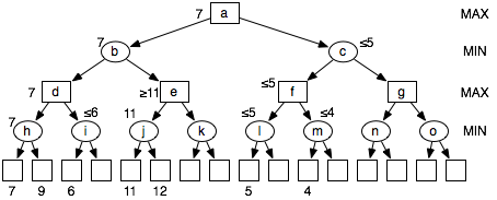
Suppose the values of the leaf nodes are given or can be computed given the definition of the game. The numbers at the bottom show some of these values. The other values are irrelevant, as we show here. Suppose we are doing a left-first depth-first traversal of this tree. The value of node h is 7, because it is the minimum of 7 and 9. Just by considering the leftmost child of i with a value of 6, we know that the value of i is less than or equal to 6. Therefore, at node d, the maximizing agent will go left. We do not have to evaluate the other child of i. Similarly, the value of j is 11, so the value of e is at least 11, and so the minimizing agent at node b will choose to go left.
The value of l is less than or equal to 5, and the value of m is less than or equal to 4; thus, the value of f is less than or equal to 5, so the value of c will be less than or equal to 5. So, at a, the maximizing agent will choose to go left. Notice that this argument did not depend on the values of the unnumbered leaves. Moreover, it did not depend on the size of the subtree that was not explored.
The previous example analyzed what can be pruned. Minimax with alpha-beta (α-β) pruning is a depth-first search algorithm that prunes by passing pruning information down in terms of parameters α and β. In this depth-first search, a node has a "current" value, which has been obtained from some of its descendants. This current value can be updated as it gets more information about the value of its other descendants.
The parameter α can be used to prune MIN nodes. Initially, it is the highest current value for all MAX ancestors of the current node. Any MIN node whose current value is less than or equal to its α value does not have to be explored further. This cutoff was used to prune the other descendants of nodes l, m, and c in the previous example.
The dual is the β parameter, which can be used to prune MAX nodes.
2: Inputs
3: N a node in a game tree
4: α,β real numbers
5: Output
6: The value for node N
7: if (N is a leaf node) then
8: return value of N
9: else if (N is a MAX node) then
10: for each child C of N do
11: Set α←max(α,MinimaxAlphaBeta(C,α,β))
12: if (α ≥ β) then
13: return β
14: return α
15: else
16: for each child C of N do
17: Set β←min(β,MinimaxAlphaBeta(C,α,β))
18: if (α ≥ β) then
19: return α
20: return β
The minimax algorithm with α-β pruning is given in Figure 10.6. It is called, initially, with
MinimaxAlphaBeta(R,-∞,∞),
where R is the root node. Note that it uses α as the current value for the MAX nodes and β as the current value for the MIN nodes.
MinimaxAlphaBeta(a,-∞,∞),
which then calls, in turn,
MinimaxAlphaBeta(b,-∞,∞)
MinimaxAlphaBeta(d,-∞,∞)
MinimaxAlphaBeta(h,-∞,∞).
This last call finds the minimum of both of its children and returns 7. Next the procedure calls
MinimaxAlphaBeta(i,7,∞),
which then gets the value for the first of i's children, which has value 6. Because α ≥ β, it returns 6. The call to d then returns 7, and it calls
MinimaxAlphaBeta(e,-∞,7).
Node e's first child returns 11 and, because α ≥ β, it returns 11. Then b returns 7, and the call to a calls
MinimaxAlphaBeta(c,7,∞),
which in turn calls
MinimaxAlphaBeta(f,7,∞),
which eventually returns 5, and so the call to c returns 5, and the whole procedure returns 7.
By keeping track of the values, the maximizing agent knows to go left at a, then the minimizing agent will go left at b, and so on.
The amount of pruning provided by this algorithm depends on the ordering of the children of each node. It works best if a highest-valued child of a MAX node is selected first and if a lowest-valued child of a MIN node is returned first. In implementations of real games, much of the effort is made to try to ensure this outcome.
Most real games are too big to carry out minimax search, even with α-β pruning. For these games, instead of only stopping at leaf nodes, it is possible to stop at any node. The value returned at the node where the algorithm stops is an estimate of the value for this node. The function used to estimate the value is an evaluation function. Much work goes into finding good evaluation functions. There is a trade-off between the amount of computation required to compute the evaluation function and the size of the search space that can be explored in any given time. It is an empirical question as to the best compromise between a complex evaluation function and a large search space.
