Third edition of Artificial Intelligence: foundations of computational agents, Cambridge University Press, 2023 is now available (including the full text).
7.3.1 Learning Decision Trees
A decision tree is a simple representation for classifying examples. Decision tree learning is one of the most successful techniques for supervised classification learning. For this section, assume that all of the features have finite discrete domains, and there is a single target feature called the classification. Each element of the domain of the classification is called a class.
A decision tree or a classification tree is a tree in which each internal (non-leaf) node is labeled with an input feature. The arcs coming from a node labeled with a feature are labeled with each of the possible values of the feature. Each leaf of the tree is labeled with a class or a probability distribution over the classes.
To classify an example, filter it down the tree, as follows. For each feature encountered in the tree, the arc corresponding to the value of the example for that feature is followed. When a leaf is reached, the classification corresponding to that leaf is returned.
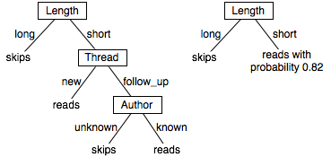
The tree on the right makes probabilistic predictions when the length is short. In this case, it predicts reads with probability 0.82 and so skips with probability 0.18.
A deterministic decision tree, in which all of the leaves are classes, can be mapped into a set of rules, with each leaf of the tree corresponding to a rule. The example has the classification at the leaf if all of the conditions on the path from the root to the leaf are true.
reads ←short ∧new.
reads ←short∧follow Up∧known.
skips ←short ∧follow Up∧unknown.
With negation as failure, the rules for either skips or reads can be omitted, and the other can be inferred from the negation.
To use decision trees as a target representation, there are a number of questions that arise:
- Given some training examples, what decision tree should be generated? Because a decision tree can represent any function of the input features, the bias that is necessary to learn is incorporated into the preference of one decision tree over another. One proposal is to prefer the smallest tree that is consistent with the data, which could mean the tree with the least depth or the tree with the fewest nodes. Which decision trees are the best predictors of unseen data is an empirical question.
- How should an agent go about building a decision tree? One way is to search the space of decision trees for the smallest decision tree that fits the data. Unfortunately the space of decision trees is enormous (see Exercise 7.7). A practical solution is to carry out a local search on the space of decision trees, with the goal of minimizing the error. This is the idea behind the algorithm described below.
