Third edition of Artificial Intelligence: foundations of computational agents, Cambridge University Press, 2023 is now available (including the full text).
6.5.2.1 Localization
Suppose a robot wants to determine its location based on its history of actions and it sensor readings. This is the problem of localization.
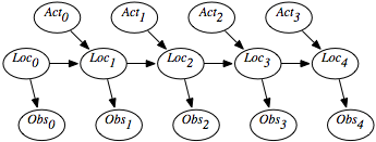
Figure 6.15 shows a belief-network representation of the localization problem. There is a variable Loci for each time i, which represents the robot's location at time i. There is a variable Obsi for each time i, which represents the robot's observation made at time i. For each time i, there is a variable Acti that represents the robot's action at time i. In this section, assume that the robot's actions are observed (we consider the case in which the robot chooses its actions in Chapter 9).
This model assumes the following dynamics: At time i, the robot is at location Loci, it observes Obsi, then it acts, it observes its action Acti, and time progresses to time i+1, where it is at location Loci+1. Its observation at time t only depends on the state at time t. The robot's location at time t+1 depends on its location at time t and its action at time t. Its location at time t+1 is conditionally independent of previous locations, previous observations, and previous actions, given its location at time t and its action at time t.
The localization problem is to determine the robot's location as a function of its observation history:
P(Loct | Obs0, Act0, Obs1, Act1, ..., Actt-1,Obst).
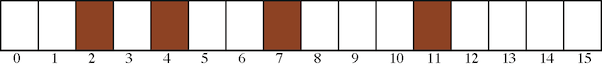
There is a circular corridor, with 16 locations numbered 0 to 15. The robot is at one of these locations at each time. This is modeled with, for every time i, a variable Loci with domain {0,1,...,15}.
- There are doors at positions 2, 4, 7, and 11 and no doors at other locations.
- The robot has a sensor that can noisily sense whether or not it is in front of a
door. This is modeled with a variable Obsi for each time
i, with domain {door,nodoor}. Assume the following conditional probabilities:
P(Obs=door | atDoor) = 0.8
P(Obs=door | notAtDoor) = 0.1where atDoor is true at states 2, 4, 7, and 11 and notAtDoor is true at the other states.
Thus, the observation is partial in that many states give the same observation and it is noisy in the following way: In 20% of the cases in which the robot is at a door, the sensor falsely gives a negative reading. In 10% of the cases where the robot is not at a door, the sensor records that there is a door.
- The robot can, at each time, move left, move right, or stay still. Assume that the
stay still action is deterministic, but the
dynamics of the moving actions are stochastic.
Just because it carries out
the goRight action does not mean that it actually goes one step
to the right - it is possible that it stays still, goes two steps right, or
even ends up at some arbitrary location (e.g., if someone picks up
the robot and moves it). Assume the following dynamics, for each
location L:
P(Loct+1= L | Actt=goRight ∧Loct=L) = 0.1
P(Loct+1= L+1 | Actt=goRight ∧Loct=L) = 0.8
P(Loct+1= L+2 | Actt=goRight ∧Loct=L) = 0.074
P(Loct+1= L' | Actt=goRight ∧Loct=L) = 0.002 for any other location L'.All location arithmetic is modulo 16. The action goLeft works the same but to the left.
The robot starts at an unknown location and must determine its location.
It may seem as though the domain is too ambiguous, the sensors are too noisy, and the dynamics is too stochastic to do anything. However, it is possible to compute the probability of the robot's current location given its history of actions and observations.
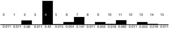
Figure 6.17 gives the robot's probability distribution over its locations, assuming it starts with no knowledge of where it is and experiences the following observations: observe door, go right, observe no door, go right, and then observe door. Location 4 is the most likely current location, with posterior probability of 0.42. That is, in terms of the network of Figure 6.15:
P(Loc2=4 | Obs0=door,Act0=goRight,Obs1=nodoor, Act1=goRight,Obs2=door)=0.42
Location 7 is the second most likely current location, with posterior probability of 0.141. Locations 0, 1, 3, 8, 12, and 15 are the least likely current locations, with posterior probability of 0.011.
You can see how well this works for other sequences of observations by using the applet at the book web site.
This is modeled in Figure 6.18 using the following variables:
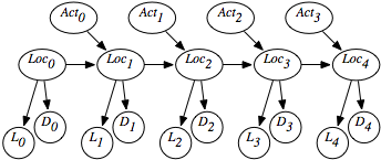
- Loct is the robot's location at time t.
- Actt is the robot's action at time t.
- Dt is the door sensor value at time t.
- Lt is the light sensor value at time t.
Conditioning on both Li and Di lets it combine information from the light sensor and the door sensor. This is an instance of sensor fusion. It is not necessary to define any new mechanisms for sensor fusion given the belief-network model; standard probabilistic inference combines the information from both sensors.
