9.1 Preferences and Utility 9.1 Preferences and Utility 9.1.2 Factored Utility

The third edition of Artificial Intelligence: foundations of computational agents, Cambridge University Press, 2023 is now available (including full text).

9.1.1 Axioms for Rationality

An agent chooses actions based on their outcomes. Outcomes are whatever the agent has preferences over. If an agent does not prefer any outcome to any other outcome, it does not matter what the agent does. Initially, we consider outcomes without considering the associated actions. Assume there are only a finite number of outcomes.

We define a preference relation over outcomes. Suppose $o_{1}$ and $o_{2}$ are outcomes. We say that $o_{1}$ is weakly preferred to outcome $o_{2}$ , written $o_{1}\succeq o_{2}$ , if outcome $o_{1}$ is at least as desirable as outcome $o_{2}$ .

Define $o_{1}\sim o_{2}$ to mean $o_{1}\succeq o_{2}$ and $o_{2}\succeq o_{1}$ . That is, $o_{1}\sim o_{2}$ means outcomes $o_{1}$ and $o_{2}$ are equally preferred. In this case, we say that the agent is indifferent between $o_{1}$ and $o_{2}$ .

Define $o_{1}\succ o_{2}$ to mean $o_{1}\succeq o_{2}$ and $o_{2}\not\succeq o_{1}$ . That is, the agent weakly prefers outcome $o_{1}$ to outcome $o_{2}$ , but does not weakly prefer $o_{2}$ to $o_{1}$ , and is not indifferent between them. In this case, we say that $o_{1}$ is strictly preferred to outcome $o_{2}$ .

Typically, an agent does not know the outcome of its actions. A lottery is defined to be a finite distribution over outcomes, written as

[p_{1}:o_{1},p_{2}:o_{2},\dots,p_{k}:o_{k}],

where each $o_{i}$ is an outcome and $p_{i}$ is a non-negative real number such that

\sum_{i}p_{i}=1.

The lottery specifies that outcome $o_{i}$ occurs with probability $p_{i}$ . In all that follows, assume that outcomes may include lotteries. This includes lotteries where the outcomes are also lotteries, and so on recursively (called lotteries over lotteries).

Axiom 9.1.

(Completeness) An agent has preferences between all pairs of outcomes:

\ o_{1}\succeq o_{2}\mbox{ or }o_{2}\succeq o_{1}.

The rationale for this axiom is that an agent must act; if the actions available to it have outcomes $o_{1}$ and $o_{2}$ then, by acting, it is explicitly or implicitly preferring one outcome over the other.

Axiom 9.2.

(Transitivity) Preferences must be transitive:

\mbox{if }o_{1}\succeq o_{2}\mbox{ and }o_{2}\succeq o_{3}\mbox{ then }o_{1}% \succeq o_{3}.

To see why this is reasonable, suppose it is false, in which case $o_{1}\succeq o_{2}$ and $o_{2}\succeq o_{3}$ and $o_{3}\succ o_{1}$ . Because $o_{3}$ is strictly preferred to $o_{1}$ , the agent should be prepared to pay some amount to get from $o_{1}$ to $o_{3}$ . Suppose the agent has outcome $o_{3}$ ; then $o_{2}$ is at least as good so the agent would just as soon have $o_{2}$ . $o_{1}$ is at least as good as $o_{2}$ so the agent would just as soon have $o_{1}$ as $o_{2}$ . Once the agent has $o_{1}$ it is again prepared to pay to get to $o_{3}$ . It has gone through a cycle of preferences and paid money to end up where it is. This cycle that involves paying money to go through it is known as a money pump because, by going through the loop enough times, the amount of money that agent must pay can exceed any finite amount. It seems reasonable to claim that being prepared to pay money to cycle through a set of outcomes is irrational; hence, a rational agent should have transitive preferences.

It follows from the transitivity and completeness axioms that transitivity holds for mixes of $\succ$ and $\succeq$ , so that if one or both of the preferences in the premise of the transitivity axiom is strict, then the conclusion is strict. That is, $\mbox{if }o_{1}\succ o_{2}\mbox{ and }o_{2}\succeq o_{3}\mbox{ then }o_{1}% \succ o_{3}$ . Also, $\mbox{if }o_{1}\succeq o_{2}\mbox{ and }o_{2}\succ o_{3}\mbox{ then }o_{1}% \succ o_{3}$ . See Exercise 1.

Axiom 9.3.

(Monotonicity) An agent prefers a larger chance of getting a better outcome than a smaller chance of getting the better outcome. That is, if $o_{1}\succ o_{2}$ and $p>q$ then

[p:o_{1},(1-p):o_{2}]\succ[q:o_{1},(1-q):o_{2}].

Note that, in this axiom, $\succ$ between outcomes represents the agent’s preference, whereas $>$ between $p$ and $q$ represents the familiar comparison between numbers.

The following axiom specifies that lotteries over lotteries only depend the outcomes and probabilities:

Axiom 9.4.

(Decomposability) (“no fun in gambling”) An agent is indifferent between lotteries that have the same probabilities over the same outcomes, even if one or both is a lottery over lotteries. For example:

	$\displaystyle[p:o_{1},$	$\displaystyle(1-p):[q:o_{2},(1-q):o_{3}]]$
		$\displaystyle\mbox{}\sim[p:o_{1},(1-p)q:o_{2},(1-p)(1-q):o_{3}].$

Also $o_{1}\sim[1:o_{1},0:o_{2}]$ for any outcomes $o_{1}$ and $o_{2}$ .

This axiom specifies that it is only the outcomes and their probabilities that define a lottery. If an agent had a preference for gambling, that would be part of the outcome space.

These four axioms imply some structure on the preference between outcomes and lotteries. Suppose that $o_{1}\succ o_{2}$ and $o_{2}\succ o_{3}$ . Consider whether the agent would prefer

•

$o_{2}$ or
•

the lottery $[p:o_{1},(1-p):o_{3}]$

for different values of $p\in[0,1]$ . When $p=1$ , the agent prefers the lottery (because, by decomposability, the lottery is equivalent to $o_{1}$ and $o_{1}\succ o_{2}$ ). When $p=0$ , the agent prefers $o_{2}$ (because the lottery is equivalent to $o_{3}$ and $o_{2}\succ o_{3}$ ). At some stage, as $p$ is varied, the agent’s preferences flip between preferring $o_{2}$ and preferring the lottery.

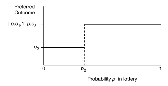
Figure 9.1: The preference between $o_{2}$ and the lottery, as a function of $p$

Figure 9.1 shows how the preferences must flip as $p$ is varied. On the $X$ -axis is $p$ and the $Y$ -axis shows which of $o_{2}$ or the lottery is preferred. The following proposition formalizes this intuition.

Proposition 9.1.

If an agent’s preferences are complete, transitive, and follow the monotonicity axiom, and if $o_{1}\succ o_{2}$ and $o_{2}\succ o_{3}$ , there exists a number $p_{2}$ such that $0\leq p_{2}\leq 1$ and

•

for all $p<p_{2}$ , the agent prefers $o_{2}$ to the lottery (i.e., $o_{2}\succ[p:o_{1},(1-p):o_{3}]$ ) and
•

for all $p>p_{2}$ , the agent prefers the lottery (i.e., $[p:o_{1},(1-p):o_{3}]\succ o_{2}$ ).

Proof.

By monotonicity and transitivity, if $o_{2}\succeq[p:o_{1},(1-p):o_{3}]$ for any $p$ then, for all $p^{\prime}<p$ , $o_{2}\succ[p^{\prime}:o_{1},(1-p^{\prime}):o_{3}]$ . Similarly, if $[p:o_{1},(1-p):o_{3}]\succeq o_{2}$ for any $p$ then, for all $p^{\prime}>p$ , $[p^{\prime}:o_{1},(1-p^{\prime}):o_{3}]\succ o_{2}$ . By completeness, for each value of $p$ , either $o_{2}\succ[p:o_{1},(1-p):o_{3}]$ , $o_{2}\sim[p:o_{1},(1-p):o_{3}]$ or $[p:o_{1},(1-p):o_{3}]\succ o_{2}$ . If there is some $p$ such that $o_{2}\sim[p:o_{1},(1-p):o_{3}]$ , then the theorem holds. Otherwise, a preference for either $o_{2}$ or the lottery with parameter $p$ implies preferences for either all values greater than $p$ or for all values less than $p$ . By repeatedly subdividing the region that we do not know the preferences for, we will approach, in the limit, a value filling the criteria for $p_{2}$ . ∎

The preceding proposition does not specify what the preference of the agent is at the point $p_{2}$ . The following axiom specifies that the agent is indifferent at this point.

Axiom 9.5.

(Continuity) Suppose $o_{1}\succ o_{2}$ and $o_{2}\succ o_{3}$ , then there exists a $p_{2}\in[0,1]$ such that

o_{2}\sim[p_{2}:o_{1},(1-p_{2}):o_{3}].

The next axiom specifies that replacing an outcome in a lottery with an outcome that is not worse, cannot make the lottery worse.

Axiom 9.6.

(Substitutability) If $o_{1}\succeq o_{2}$ then the agent weakly prefers lotteries that contain $o_{1}$ instead of $o_{2}$ , everything else being equal. That is, for any number $p$ and outcome $o_{3}$ :

[p:o_{1},(1-p):o_{3}]\succeq[p:o_{2},(1-p):o_{3}].

A direct corollary of this is that outcomes to which the agent is indifferent can be substituted for one another, without changing the preferences:

Proposition 9.2.

If an agent obeys the substitutability axiom and $o_{1}\sim o_{2}$ then the agent is indifferent between lotteries that only differ by $o_{1}$ and $o_{2}$ . That is, for any number $p$ and outcome $o_{3}$ the following indifference relation holds:

[p:o_{1},(1-p):o_{3}]\sim[p:o_{2},(1-p):o_{3}].

This follows because $o_{1}\sim o_{2}$ is equivalent to $o_{1}\succeq o_{2}$ and $o_{2}\succeq o_{1}$ , and we can use substitutability for both cases.

An agent is defined to be rational if it obeys the completeness, transitivity, monotonicity, decomposability, continuity, and substitutability axioms.

It is up to you to determine if this technical definition of rationality matches your intuitive notion of rationality. In the rest of this section, we show more consequences of this definition.

Although preferences may seem to be complicated, the following theorem shows that a rational agent’s value for an outcome can be measured by a real number. Those value measurements can be combined with probabilities so that preferences with uncertainty can be compared using expectation. This is surprising for two reasons:

•

It may seem that preferences are too multifaceted to be modeled by a single number. For example, although one may try to measure preferences in terms of dollars, not everything is for sale or easily converted into dollars and cents.
•

One might not expect that values could be combined with probabilities. An agent that is indifferent between the money $\$(px+(1-p)y)$ and the lottery $[p:\$x,\ (1-p)\$y]$ for all monetary values $x$ and $y$ and for all $p\in[0,1]$ is known as an expected monetary value (EMV) agent. Most people are not EMV agents, because they have, for example, a strict preference between $1,000,000 and the lottery $[0.5:\$0,\ 0.5:\$2,000,000]$ . (Think about whether you would prefer a million dollars or a coin toss where you would get nothing if the coin lands heads or two million if the coin lands tails.) Money cannot be simply combined with probabilities, so it may be surprising that there is a value that can be.

Proposition 9.3.

If an agent is rational, then for every outcome $o_{i}$ there is a real number $u(o_{i})$ , called the utility of $o_{i}$ , such that

•

$o_{i}\succ o_{j}$ if and only if $u(o_{i})>u(o_{j})$ and
•

utilities are linear with probabilities:

$u([p_{1}:o_{1},p_{2}:o_{2},\dots,p_{k}:o_{k}])=p_{1}u(o_{1})+p_{2}u(o_{2})+% \dots+p_{k}u(o_{k}).$

Proof.

If the agent has no strict preferences (i.e., the agent is indifferent between all outcomes) then define $u(o)=0$ for all outcomes $o$ .

Otherwise, choose the best outcome, $o_{best}$ , and the worst outcome, $o_{worst}$ , and define, for any outcome $o$ , the utility of $o$ to be the value $p$ such that

o\sim[p:o_{best},(1-p):o_{worst}].

The first part of the proposition follows from substitutability and monotonicity.

To prove the second part, any lottery can be reduced to a single lottery between $o_{best}$ and $o_{worst}$ by replacing each $o_{i}$ by its equivalent lottery between $o_{best}$ and $o_{worst}$ , and using decomposability to put it in the form $[p:o_{best},(1-p):o_{worst}]$ , with $p$ equal to $p_{1}u(o_{1})+p_{2}u(o_{2})+\cdots+p_{k}u(o_{k})$ . The details are left as an exercise. ∎

In this proof the utilities are all in the range $[0,1]$ , but any linear scaling gives the same result. Sometimes $[0,100]$ is a good scale to distinguish it from probabilities, and sometimes negative numbers are useful to use when the outcomes have costs. In general, a program should accept any scale that is intuitive to the user.

A linear relationship does not usually exist between money and utility, even when the outcomes have a monetary value. People often are risk averse when it comes to money. They would rather have $\$n$ in their hand than some randomized setup where they expect to receive $\$n$ but could possibly receive more or less.

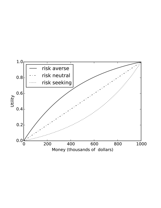
Figure 9.2: Money–utility relationships for agents with different risk profiles

Example 9.1.

Figure 9.2 shows a possible money–utility relationship for three agents. The topmost agent is risk averse, with a concave utility function. The agent with a straight-line plot is risk neutral. The lowest agent with a convex utility function is risk seeking.

The risk averse agent would rather have $300,000 than a 50% chance of getting either nothing or $1,000,000, but would prefer the gamble on the million dollars to $275,000. They would also require more than a 73% chance of winning a million dollars to prefer this gamble to half a million dollars.

For the risk-averse agent, $u(\$999000)\approx 0.9997$ . Thus, given this utility function, the risk-averse agent would be willing to pay $1000 to eliminate a $0.03\%$ chance of losing all of their money. This is why insurance companies exist. By paying the insurance company, say $600, the risk-averse agent can change the lottery that is worth $999,000 to them into one worth $1,000,000 and the insurance companies expect to pay out, on average, about $300, and so expect to make $300. The insurance company can get its expected value by insuring enough houses. It is good for both parties.

Rationality does not impose any conditions on what the utility function looks like.

Example 9.2.

Figure 9.3 shows a possible money–utility relationship for Chris who really wants a toy worth $\$30$ , but would also like one worth $\$20$ , and would like both even better. Apart from these, money does not matter much to Chris. Chris is prepared to take risks. For example, if Chris had $\$29$ , Chris would be very happy to bet $\$9$ against a single dollar of another agent on a fair bet, such as a coin toss. This is reasonable because that $9 is not much use to Chris, but the extra dollar would enable Chris to buy the $\$30$ toy. Chris does not want more than $\$60$ , because then Chris will worry about it being lost or stolen this will leave Chris open to extortion (e.g., by a sibling).

Challenges to Expected Utility

There have been a number of challenges to the theory of expected utility. The Allais Paradox, presented in 1953 [Allais and Hagen, 1979], is as follows. Which would you prefer of the following two alternatives?

A:: $\$1m$ – one million dollars
B:: lottery $[0.10:\$2.5m,0.89:\$1m,0.01:\$0]$

Similarly, what would you choose between the following two alternatives?

C:: lottery $[0.11:\$1m,0.89:\$0]$
D:: lottery $[0.10:\$2.5m,0.9:\$0]$

It turns out that many people prefer $A$ to $B$ , and prefer $D$ to $C$ . This choice is inconsistent with the axioms of rationality. To see why, both choices can be put in the same form:

A,C:: lottery $[0.11:\$1m,0.89:X]$
B,D:: lottery $[0.10:\$2.5m,0.01:\$0,0.89:X]$

In $A$ and $B$ , $X$ is a million dollars. In $C$ and $D$ , $X$ is zero dollars. Concentrating just on the parts of the alternatives that are different seems intuitive, but people seem to have a preference for certainty.

Tversky and Kahneman [1974], in a series of human experiments, showed how people systematically deviate from utility theory. One such deviation is the framing effect of a problem’s presentation. Consider the following.

•

A disease is expected to kill 600 people. Two alternative programs have been proposed:

Program A:

200 people will be saved

Program B:

with probability 1/3, 600 people will be saved, and with probability 2/3, no one will be saved

Which program would you favor?
•

A disease is expected to kill 600 people. Two alternative programs have been proposed:

Program C:

400 people will die

Program D:

with probability 1/3 no one will die, and with probability 2/3 600 will die

Which program would you favor?

Tversky and Kahneman showed that 72% of people in their experiments chose A over B, and 22% chose C over D. However, these are exactly the same choice, just described in a different way.

Prospect theory, developed by Kahneman and Tversky, is an alternative to expected utility that better fits human behavior.

Artificial Intelligence 2E

9.1.1 Axioms for Rationality

Axiom 9.1.

Axiom 9.2.

Axiom 9.3.

Axiom 9.4.

Proposition 9.1.

Proof.

Axiom 9.5.

Axiom 9.6.

Proposition 9.2.

Proposition 9.3.

Proof.

Example 9.1.

Example 9.2.

Artificial
Intelligence 2E