Artificial
Intelligence 2E
foundations of computational agents
The third edition of Artificial Intelligence: foundations of computational agents, Cambridge University Press, 2023 is now available (including full text).
3.8.1 Branch and Bound
Depth-first branch-and-bound search is a way to combine the space saving of depth-first search with heuristic information for finding optimal paths. It is particularly applicable when there are many paths to a goal. As in search, the heuristic function is non-negative and less than or equal to the cost of a lowest-cost path from to a goal node.
The idea of a branch-and-bound search is to maintain the lowest-cost path to a goal found so far, and its cost. Suppose this cost is bound. If the search encounters a path such that , path can be pruned. If a non-pruned path to a goal is found, it must be better than the previous best path. This new solution is remembered and bound is set to the cost of this new solution. The searcher then proceeds to search for a better solution.
Branch-and-bound search generates a sequence of ever-improving solutions. The final solution found is the optimal solution.
Branch-and-bound search is typically used with depth-first search, where the space saving of the depth-first search can be achieved. It can be implemented similarly to depth-bounded search, but where the bound is in terms of path cost and reduces as shorter paths are found. The algorithm remembers the lowest-cost path found and returns this path when the search finishes.
The algorithm is shown in Figure 3.12. The internal procedure cbsearch, for cost-bounded search, uses the global variables to provide information to the main procedure.
Initially, bound can be set to infinity, but it is often useful to set it to an overestimate, , of the path cost of an optimal solution. This algorithm will return an optimal solution – a lowest-cost path from the start node to a goal node – if there is a solution with cost less than the initial bound .
If the initial bound is slightly above the cost of a lowest-cost path, this algorithm can find an optimal path expanding no more arcs than search without multiple-path pruning. This happens when the initial bound is such that the algorithm prunes any path that has a higher cost than a lowest-cost path. Once it has found a path to the goal, it only explores paths whose -value is lower than the path found. These are exactly the paths that explores when it finds one solution.
If it returns when , there are no solutions. If it returns when is some finite value, it means no solution exists with cost less than . This algorithm can be combined with iterative deepening to increase the bound until either a solution is found or it can show there is no solution, using a method such as the use of hit_depth_bound in Figure 3.8. See Exercise 13.
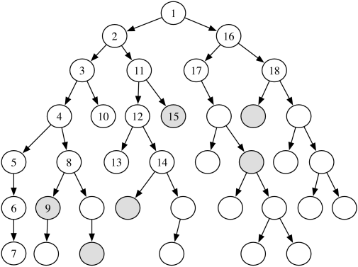
Example 3.19.
Consider the tree-shaped graph in Figure 3.13. The goal nodes are shaded. Suppose that each arc has cost 1, and there is no heuristic information (i.e., for each node ). In the algorithm, suppose and the depth-first search always selects the leftmost child first. This figure shows the order in which the nodes are checked to determine if they are a goal node. The nodes that are not numbered are not checked for being a goal node.
The subtree under the node numbered “5” does not have a goal and is explored fully (or up to depth if it had a finite value). The ninth node checked is a goal node. It has a path cost of 5, and so the bound is set to 5. From then on, only paths with a cost of less than 5 are checked for being a solution. The fifteenth node checked is also a goal. It has a path cost of 3, and so the bound is reduced to 3. There are no other goal nodes found, and so the path to the node labeled 15 is returned. It is an optimal path. There is another optimal path that is pruned; the algorithm never checks the children of the node labeled with 18.
If there were heuristic information, it could also be used to prune parts of the search space, as in search.
Cycle pruning works well with depth-first branch and bound. Multiple-path pruning is not appropriate for depth-first branch and bound because storing the explored set defeats the space saving of the depth-first search. It is possible to have a bounded size explored set, for example, by only keeping the newest elements, which will enable some pruning.