Artificial
Intelligence 2E
foundations of computational agents
The third edition of Artificial Intelligence: foundations of computational agents, Cambridge University Press, 2023 is now available (including full text).
3.3.1 Formalizing Graph Searching
A directed graph consists of
-
•
a set of nodes and
-
•
a set of arcs, where an arc is an ordered pair of nodes.
In this definition, a node could be anything. There may be infinitely many nodes and arcs. We do not assume that a graph is represented explicitly; we require only a procedure to generate nodes and arcs as needed.
The arc is an outgoing arc from and an incoming arc to .
A node is a neighbor of if there is an arc from to ; that is, if . Note that being a neighbor does not imply symmetry; just because is a neighbor of does not mean that is necessarily a neighbor of . Arcs may be labeled, for example, with the action that will take the agent from one node to another or with the cost of an action or both.
A path from node to node is a sequence of nodes such that , , and ; that is, there is an arc from to for each . Sometimes it is useful to view a path as the sequence of arcs, , or a sequence of labels of these arcs. Path is an initial part of , when .
A goal is a Boolean function on nodes. If is true, we say that node satisfies the goal, and is a goal node.
To encode problems as graphs, one node is identified as the start node. A solution is a path from the start node to a node that satisfies the goal.
Sometimes there is a cost – a non-negative number – associated with arcs. We write the cost of arc as .
The costs of arcs induce a cost of paths. Given a path , the cost of path is the sum of the costs of the arcs in the path:
An optimal solution is one of the solutions that has the lowest cost. That is, an optimal solution is a path from the start node to a goal node such that there is no path from the start node to a goal node where .
Example 3.5.
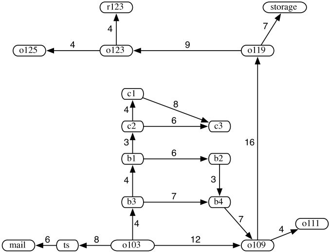
Consider the problem of the delivery robot finding a path from location to location in the domain shown in Figure 3.1. In that figure, the interesting locations are named. For simplicity, we consider only the locations shown in bold and we initially limit the directions that the robot is able to travel. Figure 3.2 shows the resulting graph where the nodes represent locations and the arcs represent possible single steps between locations. In this figure, each arc is shown with the associated cost of getting from one location to the next.
In this graph, the nodes are and the arcs are . Node has no neighbors. Node ts has one neighbor, namely mail. Node has three neighbors, namely ts, , and .
There are three paths from to :
If were the start node and were the unique goal node, each of these three paths would be a solution to the graph-searching problem. The first of these is an optimal solution, with a solution cost of .
A cycle is a nonempty path where the end node is the same as the start node – that is, such that . A directed graph without any cycles is called a directed acyclic graph (DAG). Note that this should be called an acyclic directed graph, because it is a directed graph that happens to be acyclic, not an acyclic graph that happens to be directed, but DAG sounds better than ADG!
A tree is a DAG where there is one node with no incoming arcs and every other node has exactly one incoming arc. The node with no incoming arcs is called the root of the tree. A node with no outgoing arcs is called a leaf. In a tree, neighbors are often called children, and we use the family-tree metaphor, with grandparents, siblings, and so on.
In many problems the search graph is not given explicitly, but is dynamically constructed as needed. For the search algorithms, all that is required is a way to generate the neighbors of a node and to determine if a node is a goal node.
The forward branching factor of a node is the number of outgoing arcs from the node. The backward branching factor of a node is the number of incoming arcs to the node. These factors provide measures for the complexity of graph algorithms. When we discuss the time and space complexity of the search algorithms, we assume that the branching factors are bounded, meaning they are all less than some postive integer.
Example 3.6.
In the graph of Figure 3.2, the forward branching factor of node is three because there are three outgoing arcs from node . The backward branching factor of node is zero; there are no incoming arcs to node . The forward branching factor of mail is zero and the backward branching factor of mail is one. The forward branching factor of node is two and the backward branching factor of is one.
The branching factor is an important key component in the size of the graph. If the forward branching factor for each node is , and the graph is a tree, there are nodes that are arcs away from the start node.