Artificial
Intelligence 2E
foundations of computational agents
The third edition of Artificial Intelligence: foundations of computational agents, Cambridge University Press, 2023 is now available (including full text).
10.4 Bayesian Learning
Rather than choosing the most likely model or delineating the set of all models that are consistent with the training data, another approach is to compute the posterior probability of each model given the training examples.
The idea of Bayesian learning is to compute the posterior probability distribution of the target features of a new example conditioned on its input features and all the training examples.
Suppose a new case has inputs (which we write simply as ) and target features . The aim is to compute , where is the set of training examples. This is the probability distribution of the target variables given the particular inputs and the examples. The role of a model is to be the assumed generator of the examples. If we let be a set of disjoint and covering models, then reasoning by cases and the chain rule give
The first two equalities follow from the definition of conditional probability. The last equality relies on two assumptions: the model includes all the information about the examples that is necessary for a particular prediction, , and the model does not change depending on the inputs of the new example, . Instead of choosing the best model, Bayesian learning relies on model averaging, averaging over the predictions of all the models, where each model is weighted by its posterior probability given the training examples.
can be computed using Bayes’ rule:
Thus, the weight of each model depends on how well it predicts the data (the likelihood) and its prior probability. The denominator, , is a normalizing constant to make sure the posterior probabilities of the models sum to 1. is called the partition function. Computing may be very difficult when there are many models.
A set of examples are independent and identically distributed (i.i.d.), given model if examples and , for , are independent given . If the set of training examples is , the assumption that the examples are i.i.d. implies
The i.i.d. assumption can be represented as a belief network, shown in Figure 10.10, where each of the are independent given model .
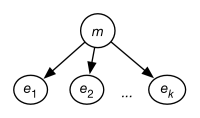
If is made into a discrete variable, any of the inference methods of the previous chapter could be used for inference in this network. A standard reasoning technique in such a network is to condition on every observed and to query the model variable or an unobserved variable.
The set of models may include structurally different models in addition to models that differ in the values of the parameters. One of the techniques of Bayesian learning is to make the parameters of the model explicit and to determine the distribution over the parameters.
Example 10.14.
Consider the simplest learning task of learning a single Boolean random variable, , with no input features. (This is the case covered in Section 7.2.3.) Each example specifies or . The aim is to learn the probability distribution of given the set of training examples.
There is a single parameter, , that determines the set of all models. Suppose that represents the probability of . We treat as a real-valued random variable on the interval . Thus, by definition of , and .
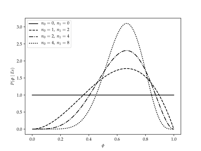
Suppose, first, an agent has no prior information about the probability of Boolean variable and no knowledge beyond the training examples. This ignorance can be modeled by having the prior probability distribution of the variable as a uniform distribution over the interval . This is the probability density function labeled in Figure 10.11.
We can update the probability distribution of given some examples. Assume that the examples, obtained by running a number of independent experiments, are a particular sequence of outcomes that consists of cases where is false and cases where is true.
The posterior distribution for given the training examples can be derived by Bayes’ rule. Let the examples be the particular sequence of observations that resulted in occurrences of and occurrences of . Bayes’ rule gives us
The denominator is a normalizing constant to make sure the area under the curve is 1.
Given that the examples are i.i.d.,
because there are cases where , each with a probability of , and cases where , each with a probability of .
Note that is the particular sequence of observations made. If the observation was just that there were a total of occurrences of and occurrences of , we would get an different answer, because we would have to take into account all the possible sequences that could have given this count. The latter is known as the binomial distribution.
One possible prior probability, , is a uniform distribution on the interval . This would be reasonable when the agent has no prior information about the probability.
Figure 10.11 gives some posterior distributions of the variable based on different sample sizes, and given a uniform prior. The cases are , , and . Each of these peak at the same place, namely at . More training examples make the curve sharper.
The distribution of this example is known as the beta distribution; it is parameterized by two counts, and , and a probability . Traditionally, the parameters for the beta distribution are one more than the counts; thus, . The beta distribution is
where is a normalizing constant that ensures the integral over all values is 1. Thus, the uniform distribution on is the beta distribution .
Suppose instead that is a discrete variable with different values. The generalization of the beta distribution to cover this case is known as the Dirichlet distribution. The Dirichlet distribution with two sorts of parameters, the “counts” , and the probability parameters , is
where is the probability of the th outcome (and so ) and is a non-negative real and is a normalizing constant that ensures the integral over all the probability values is 1. We can think of as one more than the count of the th outcome, . The Dirichlet distribution looks like Figure 10.11 along each dimension (i.e., as each varies between 0 and 1).
For many cases, averaging over all models weighted by their posterior distribution is difficult, because the models may be complicated (e.g., if they are decision trees or even belief networks). For the Dirichlet distribution, the expected value for outcome (averaging over all ) is
The reason that the parameters are one more than the counts in the definitions of the beta and Dirichlet distributions is to make this formula simple. This fraction is well defined only when the are all non-negative and not all are zero.
Example 10.15.
Consider Example 10.14, which determines the value of based on a sequence of observations made up of cases where is false and cases where is true. Consider the posterior distribution as shown in Figure 10.11. What is interesting about this is that, whereas the most likely posterior value of is , the expected value of this distribution is .
Thus, the expected value of the curve is , for the case the expected value is , and for the case it is . As the learner gets more training examples, this value approaches .
This estimate is better than for a number of reasons. First, it tells us what to do if the learning agent has no examples: use the uniform prior of . This is the expected value of the case. Second, consider the case where and . The agent should not use , because this says that is impossible, and it certainly does not have evidence for this! The expected value of this curve with a uniform prior is .
An agent does not have to start with a uniform prior; it could start with any prior distribution. If the agent starts with a prior that is a Dirichlet distribution, its posterior will be a Dirichlet distribution. The posterior distribution can be obtained by adding the observed counts to the parameters of the prior distribution.
Thus, the beta and Dirichlet distributions provide a justification for using pseudocounts for estimating probabilities. The pseudocount represents the prior knowledge. A flat prior gives a pseudocount of 1. Thus, Laplace smoothing can be justified in terms of making predictions from initial ignorance.
In addition to using the posterior distribution of to derive the expected value, we can use it to answer other questions such as: What is the probability that the posterior probability, , is in the range ? In other words, derive . This is the problem that the Reverend Thomas Bayes solved more than 250 years ago [Bayes, 1763]. The solution he gave – although in much more cumbersome notation – was
This kind of knowledge is used in surveys when it may be reported that a survey is correct with an error of at most , times out of . It is also the same type of information that is used by probably approximately correct (PAC) learning, which guarantees an error at most at least of the time. If an agent chooses the midpoint of the range , namely , as its hypothesis, it will have error less than or equal to , just when the hypothesis is in . The value corresponds to . If and , choosing the midpoint will result in an error at most in of the time. PAC learning gives worst-case results, whereas Bayesian learning gives the expected number. Typically, the Bayesian estimate is more accurate, but the PAC results give a guarantee of a bound on the error. The sample complexity, the number of samples required to obtain some given accuracy, for Bayesian learning is typically much less than that of PAC learning – many fewer examples are required to expect to achieve the desired accuracy than are needed to guarantee the desired accuracy.