A hidden variable or latent variable is a probabilistic variable that is not observed in a data set. A Bayes classifier can be the basis for unsupervised learning by making the class a hidden variable.

The expectation maximization or EM algorithm can be used to learn probabilistic models with hidden variables. Combined with a naive Bayes classifier, it does soft clustering, similar to the $k$-means algorithm, but where examples are probabilistically in classes.

As in the $k$-means algorithm, the training examples and the number of classes, $k$, are given as input.

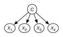Given the data, a naive Bayes model is constructed where there is a variable for each feature in the data and a hidden variable for the class. The class variable is the only parent of the other features. This is shown in Figure 10.4. The class variable has domain $\{1,2,\mathrm{\dots },k\}$ where $k$ is the number of classes. The probabilities needed for this model are the probability of the class $C$ and the probability of each feature given $C$. The aim of the EM algorithm is to learn probabilities that best fit the data.

The EM algorithm conceptually augments the data with a class feature, $C$, and a count column. Each original example gets mapped into $k$ augmented examples, one for each class. The counts for these examples are assigned so that they sum to 1. For example, for four features and three classes, we could have

The EM algorithm repeats the two steps:

• •

  E step: Update the augmented counts based on the probability distribution. For each example in the original data, the count associated with in the augmented data is updated to

  $$P(C=c\mid X_1=v_1,\mathrm{\dots },X_n=v_n).$$

  Note that this step involves probabilistic inference. This is an expectation step because it computes the expected values.

• •

  M step: Infer the probabilities for the model from the augmented data. Because the augmented data has values associated with all the variables, this is the same problem as learning probabilities from data in a naive Bayes classifier. This is a maximization step because it computes the maximum likelihood estimate or the maximum a posteriori probability (MAP) estimate of the probability.

The EM algorithm starts with random probabilities or random counts. EM will converge to a local maximum of the likelihood of the data.

This algorithm returns a probabilistic model, which is used to classify an existing or new example. An example is classified using

The algorithm does not need to store the augmented data, but maintains a set of sufficient statistics, which is enough information to compute the required probabilities. In each iteration, it sweeps through the data once to compute the sufficient statistics. The sufficient statistics for this algorithm are

• •

  $cc$, the class count, a $k$-valued array such that $cc[c]$ is the sum of the counts of the examples in the augmented data with $class=c$

• •

  $fc$, the feature count, a three-dimensional array such that $fc[i,v,c]$, for $i$ from 1 to $n$, for each value $v$ in $domain(X_i)$, and for each class $c$, is the sum of the counts of the augmented examples $t$ with $X_i(t)=val$ and $class(t)=c$.

The sufficient statistics from the previous iteration are used to infer the new sufficient statistics for the next iteration. Note that $cc$ could be computed from $fc$, but it is easier to maintain $cc$ directly.

The probabilities required of the model can be computed from $cc$ and $fc$:

where $\left|E\right|$ is the number of examples in the original data set (which is the same as the sum of the counts in the augmented data set).

Figure 10.6 gives the algorithm to compute the sufficient statistics, from which the probabilities are derived as above. Evaluating $P(C=c\mid X_1=v_1,\mathrm{\dots },X_n=v_n)$ in line 17 relies on the counts in $cc$ and $fc$. This algorithm has glossed over how to initialize the counts. One way is for $P(C\mid X_1=v_1,\mathrm{\dots },X_n=v_n)$ to return a random distribution for the first iteration, so the counts come from the data. Alternatively, the counts can be assigned randomly before seeing any data. See Exercise 6.

The algoritm will eventually converge when $cc$ and $fc$ do not change much in an iteration. The threshold for the approximately equal in line 21 can be tuned to trade off learning time and accuracy. An alternative is to run the algorithms for a fixed number of iterations.

Notice the similarity with the $k$-means algorithm. The E step (probabilistically) assigns examples to classes, and the M step determines what the classes predict.

Note that, as long as $k>1$, EM virtually always has multiple local maxima. In particular, any permutation of the class labels of a local maximum will also be a local maximum. To try to find a global maximum, multiple restarts can be tried, and the model with the lowest log-likelihood returned.