Artificial
Intelligence 3E
foundations of computational agents
3.7 Pruning the Search Space
The preceding algorithms can be improved by taking into account multiple paths to a node. The following presents two pruning strategies. The simplest strategy is to prune cycles; if the goal is to find a least-cost path, it is useless to consider paths with cycles. The other strategy is only ever to consider one path to a node and to prune other paths to that node.
3.7.1 Cycle Pruning
A graph representing a search space may include cycles. For example, in the robot delivery domain of Figure 3.10, the robot can go back and forth between nodes and . Some of the search methods presented so far can get trapped in cycles, continuously repeating the cycle and never finding an answer even in finite graphs. The other methods can loop through cycles, wasting time, but eventually still find a solution.
A simple method of pruning the search, while guaranteeing that a solution will be found in a finite graph, is to ensure that the algorithm does not consider neighbors that are already on the path from the start. Cycle pruning, or loop pruning, checks whether the last node on the path already appears earlier on the path from the start node to that node. A path , where , is not added to the frontier at line 16 of Figure 3.5 or is discarded when removed from the frontier.
The computational complexity of cycle pruning depends on which search method is used. For depth-first methods, the overhead can be as low as a constant factor, by storing the elements of the current path as a set (e.g., by maintaining a bit that is set when the node is in the path, or using a hash function). For the search strategies that maintain multiple paths – namely, all of those with exponential space in Figure 3.18 – cycle pruning takes time linear in the length of the path being searched. These algorithms cannot do better than searching up the partial path being considered, checking to ensure they do not add a node that already appears in the path.
3.7.2 Multiple-Path Pruning
There is often more than one path to a node. If only one path is required, a search algorithm can prune from the frontier any path that leads to a node to which it has already found a path.
Multiple-path pruning is implemented by maintaining an explored set (traditionally called the closed list) of nodes that are at the end of paths that have been expanded. The explored set is initially empty. When a path is selected, if is already in the explored set, the path can be discarded. Otherwise, is added to the explored set, and the algorithm proceeds as before. See Figure 3.16.
This approach does not necessarily guarantee that the least-cost path is not discarded. Something more sophisticated may have to be done to guarantee that an optimal solution is found. To ensure that the search algorithm can still find a lowest-cost path to a goal, one of the following can be done:
-
•
Make sure that the first path found to any node is a lowest-cost path to that node, then prune all subsequent paths found to that node.
-
•
If the search algorithm finds a lower-cost path to a node than one already found, it could remove all paths that used the higher-cost path to the node (because these cannot be on an optimal solution). That is, if there is a path on the frontier , and a path to is found that has a lower cost than the portion of the path from to in , then can be removed from the frontier.
-
•
Whenever the search finds a lower-cost path to a node than a path to that node already found, it could incorporate a new initial section on the paths that have extended the initial path. Thus, if there is a path on the frontier, and a path to is found with a cost lower than the portion of from to , then can replace the initial part of to .
The first of these alternatives allows the use of the explored set without losing the ability to find an optimal path. The others require more sophisticated algorithms.
In lowest-cost-first search, the first path found to a node (i.e., when the node is selected from the frontier) is the lowest-cost path to the node. Pruning subsequent paths to that node cannot remove a lower-cost path to that node, and thus pruning subsequent paths to each node still enables an optimal solution to be found.
does not guarantee that when a path to a node is selected for the first time it is the lowest-cost path to that node. Note that the admissibility theorem guarantees this for every path to a goal node but not for every path to any node. Whether it holds for all nodes depends on properties of the heuristic function.
A consistent heuristic is a non-negative function on nodes, such that for any two nodes and , where is the cost of the least-cost path from to . As for any goal , a consistent heuristic is never an overestimate of the cost of going from a node to a goal.
Consistency can be guaranteed if the heuristic function satisfies the monotone restriction: for any arc . It is easier to check the monotone restriction as it only depends on the arcs, whereas consistency depends on all pairs of nodes.
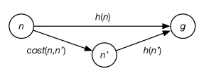
Consistency and the monotone restriction can be understood in terms of the triangle inequality, which specifies that the length of any side of a triangle cannot be greater than the sum of lengths of the other two sides. In consistency, the estimated cost of going from to a goal should not be more than the estimated cost of first going to then to a goal (see Figure 3.17).
Euclidean distance – the straight-line distance in a multidimensional space – satisfies the triangle inequality. Therefore, when the cost function is the Euclidean distance, the heuristic function that is the shortest distance between node and a goal satisfies the monotone restriction and so is consistent. A heuristic function that is a solution to a simplified problem that has shorter solutions also typically satisfies the monotone restriction and so is consistent.
With the monotone restriction, the -values of the paths selected from the frontier are monotonically non-decreasing. That is, when the frontier is expanded, the -values do not get smaller.
Proposition 3.2.
With a consistent heuristic, multiple-path pruning can never prevent search from finding an optimal solution.
That is, under the conditions of Proposition 3.1, which guarantee finds an optimal solution, if the heuristic function is consistent, with multiple-path pruning will always find an optimal solution.
Proof.
The gist of the proof is to show that if the heuristic is consistent, when expands a path to a node , no other path to can have a lower cost than . Thus, the algorithm can prune subsequent paths to any node and will still find an optimal solution.
Let’s use a proof by contradiction. Suppose the algorithm has selected a path to node for expansion, but there exists a lower-cost path to node , which it has not found yet. Then there must be a path on the frontier that is the initial part of the lower-cost path to . Suppose path ends at node . It must be that , because was selected before . This means that
If the path to via has a lower cost than the path , then
where is the actual cost of a lowest-cost path from node to . From these two equations, it follows that
where the last inequality follows because is defined to be . This cannot happen if , which is the consistency condition. ∎
search in practice includes multiple-path pruning; if is used without multiple-path pruning, the lack of pruning should be made explicit. It is up to the designer of a heuristic function to ensure that the heuristic is consistent, and so an optimal path will be found.
Multiple-path pruning subsumes cycle pruning, because a cycle is another path to a node and is therefore pruned. Multiple-path pruning can be done in constant time, by setting a bit on each node to which a path has been found if the graph is explicitly stored, or using a hash function. Multiple-path pruning is preferred over cycle pruning for breadth-first methods where virtually all of the nodes considered have to be stored anyway.
Depth-first search does not have to store all of the nodes at the end of paths already expanded; storing them in order to implement multiple-path pruning makes depth-first search exponential in space. For this reason, cycle pruning is preferred over multiple-path pruning for algorithms based on depth-first search, including depth-first branch and bound. It is possible to have a bounded size explored set, for example, by only keeping the newest elements, which enables some pruning without the space explosion.
3.7.3 Summary of Search Strategies
Figure 3.18 summarizes the search strategies presented so far.
| Strategy | Selection from frontier | Path found | Space |
|---|---|---|---|
| Breadth-first | First node added | Fewest arcs | |
| Depth-first | Last node added | ✘ | |
| Iterative deepening | N/A | Fewest arcs | |
| Greedy best-first | Minimal | ✘ | |
| Lowest-cost-first | Minimal | Least cost | |
| Minimal | Least cost | ||
| DF B&B | N/A | Least cost |
“Selection from frontier” refers to which element is selected in line 13 of the generic graph-searching algorithm of Figure 3.5. Iterative deepening and depth-first branch and bound (DF B&B) are not instances of the generic search algorithm, and so the selection from the frontier is not applicable.
“Path found” refers to guarantees about the path found (for graphs with finite branching factor and arc costs bounded above zero). “✘” means the strategy is not guaranteed to find a path. Depth-first branch and bound (DF B&B) requires an initial finite bound that is greater than the cost of a least-cost solution.
“Space” refers to the worst-case space complexity; , the depth, is the maximum number of arcs in a path expanded before a solution is found, and is a bound on the branching factor.
Lowest-cost-first, , and depth-first branch-and-bound searches are guaranteed to find a lowest-cost solution, as long as the conditions of Proposition 3.1 hold, even if the graph is infinite. Breadth-first search and iterative deepening will find a path with the fewest arcs as long as each node has a finite branching factor. Depth-first search and greedy best-first searches, when the graph is infinite or when there is no cycle pruning or multiple path pruning, sometimes do not halt, even if a solution exists.
A search algorithm is complete if it is guaranteed to find a solution if there is one. Those search strategies that are guaranteed to find a path with fewest arcs or the least cost are complete. They have worst-case time complexity which increases exponentially with the number of arcs on the paths explored. There can only be algorithms that are complete but better than exponential time complexity if , which is not expected to be true. The algorithms that are not guaranteed to halt (depth-first and greedy best-first) have an infinite worst-case time complexity.
Depth-first search uses linear space with respect to the length of the longest path explored, but is not guaranteed to find a solution even if one exists. Breadth-first, lowest-cost-first, and may be exponential in both space and time, but are guaranteed to find a solution if one exists, even if the graph is infinite as long as there are finite branching factors and arc costs are bounded above zero. Iterative deepening reduces the space complexity at the cost of recomputing the elements on the frontier. Depth-first branch and bound (DF B&B) reduces the space complexity, but can search more of the space or fail to find a solution, depending on the initial bound.
Artificial Intelligence: Foundations of Computational Agents, Poole
& Mackworth
Copyright © 2023, David L. Poole and Alan K. Mackworth. 
This work is licensed under a Creative Commons Attribution-NonCommercial-NoDerivatives 4.0 International License.