Artificial
Intelligence 3E
foundations of computational agents
14.7 Multiagent Reinforcement Learning
14.7.1 Perfect-Information Games
For a perfect-information game, where agents take turns and observe the state of the world before acting, and each agent acts to maximize its own utility, the single-agent reinforcement learning algorithms of Chapter 13 can work unchanged. Each agent can assume that the other agents are part of the environment. This works whether the opponent is playing its optimal strategy or is also learning. The reason this works is that there is a unique Nash equilibrium which is the value for the agent of the current node in the game tree. This strategy is the best response to the other agents.
If the opponent is not playing its optimal strategy or converging to an optimal strategy, a learning agent could converge to a non-optimal strategy. It is possible for an opponent to train a learning agent to carry out a non-optimal strategy by playing badly, and then for the opponent to change to another strategy in order to exploit the agent’s sub-optimal strategy. However, the learning agent could then learn from the (now) better opponent.
It is possible to use reinforcement learning to simulate both players in a game, and to learn for both. For two-player, zero-sum, perfect-information games, as in minimax, the game can be characterized by a single value that one agent is trying to minimize and the other is trying to maximize. In that case, an agent could learn , an estimate of this value for being in state and carrying out action . The algorithms can remain essentially the same, but need to know which player’s turn it is, and the Q-value would then be updated by maximizing or minimizing depending on which player’s turn it is.
14.7.2 Reinforcement Learning with Stochastic Policies
For multiple agents with imperfect information, including simultaneous action games, it is possible that there are multiple Nash equilibria, and that no deterministic strategy is optimal. Due to the existence of multiple equilibria, in many cases it is not clear what an agent should actually do, even if it knows all of the outcomes for the game and the utilities of the agents. However, most real strategic encounters are much more difficult, because the agents do not know the outcomes or the utilities of the other agents.
For games where the only Nash equilibria consist of randomized strategies, such as in the soccer penalty kick (Figure 14.8), learning any deterministic policy is not a good idea because any deterministic strategy can be exploited by the other agent. For other games with multiple Nash equilibria, such as those explored in Section 14.4, agents may need to play multiple games to coordinate on a strategy profile where neither wants to deviate.
Reinforcement learning can be extended to such situations by explicitly representing stochastic policies, which are policies that specify a probability distribution over actions. This automatically allows for a form of exploration, because any action with a non-zero probability will be tried repeatedly.
This section presents a variant of SARSA, where each player represents a stochastic policy using counts for each action, as in a Dirichlet distribution. The agent updates the counts of its actions based on the rewards received.
The stochastic policy iteration controller of Figure 14.10 is similar to the SARSA algorithm but learns a stochastic policy, a probability distribution over actions for each state. The policy is represented in as counts, as in a Dirichlet distribution, over which action has highest value (plus pseudo counts). The stochastic policy is obtained by normalizing the array, so that the probability of doing action in state is
The algorithm is the same as SARSA, except that it updates by adding one to the value for an action with highest estimated -value.
To trade off exploration and exploitation, is initialized with counts that are not close to zero (e.g., 5 is used in the examples below) so that one policy does not become dominant quickly and/or by initializing with a high value to encourage explorations. An open-source implementation of this learning controller is available from AIPython (aipython.org).
If there is a unique Nash equilibrium in pure strategies, and all of the agents use this algorithm, they will converge to this equilibrium. Dominated strategies will have their probability converge to zero. In Example 14.15, it will find the Nash equilibrium. Similarly for the prisoner’s dilemma in Example 14.13, it will converge to the unique equilibrium where both agents take. Thus, this algorithm does not learn to cooperate, where cooperating agents will both give in the prisoner’s dilemma to maximize their payoffs.
If there are multiple pure equilibria, this algorithm will converge to one of them. The agents thus learn to coordinate. For example, in the football–shopping game of Example 14.12, it will converge to one of the equilibria of both shopping or both going to the football game.
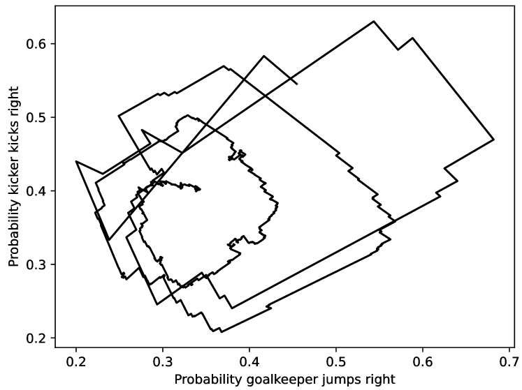
A plot of the policy of two players using the stochastic reinforcement learning algorithm of Figure 14.10 (with having a single element, , , , ) for the soccer penalty kick of Example 14.9.
After the first action, the policy is the position (0.455, 0.545) and follows the line, ending up at the point (0.338, 0.399). The Nash equilibrium is the point (0.3, 0.4), as derived in Example 14.16.
Example 14.20.
Consider the penalty kick game of Example 14.9. Figure 14.11 shows a plot of two players using the learning algorithm for Example 14.9. This figure plots the probabilities for the goalkeeper jumping right and the kicker kicking right for one run of the learning algorithm. That is, it shows the value for the normalized function. In this run, is initialized to 1, and the counts in are initialized to 5. At equilibrium, the kicker kicks right with probability 0.4 and the goalkeeper jumps right with probability 0.3.
Consider a two-agent competitive game where there is only a randomized Nash equilibrium. If agents and are competing and agent is playing a Nash equilibrium, it does not matter which action in its support set is performed by agent ; they all have the same value to . This algorithm tends to find a Nash equilibrium, and then one agent diverges from the equilibrium because there is no penalty for doing so when the other agent is playing an equilibrium strategy. After the agent deviates, the other can change its strategy to exploit the deviation. This is one explanation for the cycling behavior.
There are many variants of this algorithm, including weighting more recent experiences more than older ones, adjusting the probabilities by a constant (being careful to ensure the probabilities are between 0 and 1 and sum to 1). See Exercise 14.9.
An agent using this algorithm does not need to know the game or the payoffs. When an agent knows the game, another simple strategy is fictitious play, where the agent collects the statistics of the other player and, assuming those statistics reflect the stochastic policy of the other agent, plays a best response. Both players using fictitious play converges to a Nash equilibrium for many types of games (including two-player zero-sum games).
Note that there is no perfect learning strategy. If an opposing agent knew the exact strategy (whether learning or not) agent was using, and could predict what agent would do, it could exploit that knowledge.
Example 14.21.
Suppose two agents are playing the penalty kick game (Example 14.9) and one agent (Agent 1) is using fictitious play. Agent 1 has a deterministic strategy (except for a few cases). The opposing player, Agent 2, if they know Agent 1 is using fictitious play, could predict what Agent 1 is going to do, and carry out the best response. They will almost always be able to beat Agent 1.
The only time Agent 2 is not guaranteed to beat Agent 1 is when Agent 2’s history corresponds to a Nash equilibrium, in which case Agent 1 could be stochastic. In that case, at the next step, Agent 2 will have a different ratio, and so will not be playing an equilibrium strategy, and then can beat Agent 1.
This property is not a feature of fictitious play. Indeed, if Agent 1 can convince Agent 2 that Agent 1 is using fictitious play, then Agent 1 could predict what Agent 2 will do, and play to beat that. Agent 2, if they consider the hypothesis that Agent 1 is not actually using fictitious play, should be able to determine that Agent 1 is not using fictitious play, and change their strategy.
14.7.3 State-of-the-Art Game Players
In 2016 the computer program AlphaGo beat Lee Sedol, one of the top Go players in the world, in a five-game Go match. AlphaZero, the follow-on program with zero programmed prior knowledge of the games – beyond a simulator of the games – plays world-class chess, shogi, and Go. The main features of AlphaZero are:
-
•
It implements modified policy iteration, using a deep neural network with the board position as the input and the output is both the value function (the expected value with for a win, 0 for a draw, and for a loss) and a stochastic policy (a probability distribution using softmax over the possible moves, incorporating the upper confidence bound). The parameters of the neural network are optimized with respect to the sum of the squared loss of the value function, the log loss of the distribution representing the stochastic policy, and an L2 regularization term.
-
•
At each step, it carries out a stochastic simulation – forward sampling, as there are no observations – of the rest of the game, following the stochastic policy. This stochastic simulation is used to estimate the expected value of each action. This is known as Monte Carlo tree search (MCTS). Note that MCTS relies on a model; it has to be able to restart the search from any point.
-
•
It was trained on self-play, playing itself for tens of millions of games, using first and second-generation tensor processing units as the hardware.
Artificial Intelligence: Foundations of Computational Agents, Poole
& Mackworth
Copyright © 2023, David L. Poole and Alan K. Mackworth. 
This work is licensed under a Creative Commons Attribution-NonCommercial-NoDerivatives 4.0 International License.