Artificial
Intelligence 3E
foundations of computational agents
14.3 Solving Perfect Information Games
Fully observable with multiple agents is typically called perfect information. In perfect-information games, agents act sequentially and, when an agent has to act, it gets to observe the state of the world before deciding what to do. Each agent acts to maximize its own utility.
A perfect-information game can be represented as an extensive-form game where the information sets all contain a single node. They can also be represented as a multiagent decision network where the decision nodes are totally ordered and, for each decision node, the parents of that decision node include the preceding decision node and all of their parents (so they are a multiagent counterpart of no-forgetting decision networks).
Perfect-information games are solvable in a manner similar to fully observable single-agent systems. They can be solved backward, from the last decisions to the first, using dynamic programming, or forward using search. The multiagent algorithm maintains a utility for each agent and, for each move, it selects an action that maximizes the utility of the agent making the move. The dynamic programming variant, called backward induction, starts from the end of the game, computing and caching the values and the plan of each node for each agent.
Figure 14.5 gives a top-down, depth-first search algorithm for evaluating a game tree for a perfect information game. It enumerates the whole tree. At each internal node, the agent that controls the node selects a child that is best for it. This arbitrarily chooses the first child that maximizes the agent’s score (the on line 12), but as the following example shows, which one is selected can affect the utility.
Example 14.6.
Consider the sharing game of Figure 14.2. In the recursive calls, Barb gets to choose the value that maximizes her utility. Thus, she will choose “yes” for the right two nodes she controls, and would choose either for the leftmost node she controls. Suppose she chooses “no” for this node, then Andy gets to choose one of his actions: has utility 0 for him, has utility 1, and has utility 0, so he chooses to share. If Barb had chosen “yes” for the leftmost node, Andy would keep, and so Andy would get both items.
14.3.1 Adversarial Games
The case where two agents are competing, so that a positive reward for one is a negative reward for the other, is a two-agent zero-sum game. An agent that plays such a game well requires adversarial reasoning. The value of such a game can be characterized by a single number that one agent is trying to maximize and the other agent is trying to minimize, which leads to a minimax search space. Each node is either a MAX node, if it is controlled by the agent trying to maximize, or a MIN node, if it is controlled by the agent trying to minimize.
Figure 14.5 implements a minimax algorithm for zero-sum perfect information games, by the MAX agent choosing an action with the maximum value, and the MIN agent choosing an action with the maximum of the negation of the value.
The game-tree search of Figure 14.5 traverses the whole game tree. It is possible to prune part of the search tree for minimax games by showing that some part of the tree will never be part of an optimal play.
Example 14.7.
Consider searching in the game tree of Figure 14.6. In this figure, the square MAX nodes are controlled by the maximizing agent, and the round MIN nodes are controlled by the minimizing agent.
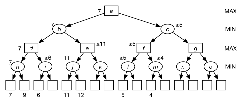
Suppose the values of the leaf nodes are given or are computed given the definition of the game. The numbers at the bottom show some of these values. The other values are irrelevant, as shown here. Suppose you are doing a left-first, depth-first traversal of this tree. The value of node is 7, because it is the minimum of 7 and 9. Just by considering the leftmost child of with a value of , you know that the value of is less than or equal to 6. Therefore, at node , the maximizing agent will go left. You do not have to evaluate the other child of . Similarly, the value of is 11, so the value of is at least 11, and so the minimizing agent at node will choose to go left.
The value of is less than or equal to 5, and the value of is less than or equal to 4; thus, the value of is less than or equal to , so the value of will be less than or equal to 5. So, at , the maximizing agent will choose to go left. Notice that this argument did not depend on the values of the unnumbered leaves. Moreover, it did not depend on the size of the subtrees that were not explored.
The previous example analyzed what can be pruned. Minimax with alpha–beta (–) pruning is a depth-first search algorithm that prunes by passing pruning information down in terms of parameters and . In this depth-first search, a node has a score, which has been obtained from (some of) its descendants.
The parameter is used to prune MIN nodes. Initially, it is the highest current value for all MAX ancestors of the current node. Any MIN node whose current value is less than or equal to its value does not have to be explored further. This cutoff was used to prune the other descendants of nodes , , and in the previous example.
The parameter is used to prune MAX nodes in an analogous way.
The minimax algorithm with – pruning is given in Figure 14.7. It is called, initially, with , where is the root node. It returns a pair of the value for the node and a path of choices that lead to this value. (Note that this path does not include .) Line 13 performs pruning; at this stage the algorithm knows that the current path will never be chosen, and so returns a current score. Similarly, line 22 performs -pruning. Line 17 and line 26 concatenate to the path, as it has found a best path for the agent. In this algorithm, the path “” is sometimes returned for non-leaf nodes; this only occurs when the algorithm has determined this path will not be used.
Example 14.8.
Consider running on the tree of Figure 14.6. Consider the recursive calls (and the values returned, but not the paths). Initially, it calls
which then calls, in turn:
This last call finds the minimum of both of its children and returns . Next the procedure calls
which then gets the value for the first of ’s children, which has value . Because , it returns . The call to then returns , and it calls
Node ’s first child returns and, because , it returns . Then returns , and the call to calls
which in turn calls
which eventually returns 5, and so the call to returns 5, and the whole procedure returns 7.
By keeping track of the values, the maximizing agent knows to go left at , then the minimizing agent will go left at , and so on.
The amount of pruning provided by this algorithm depends on the ordering of the children of each node. It works best if a highest-valued child of a MAX node is selected first and if a lowest-valued child of a MIN node is returned first. In implementations of real games, much of the effort is made to try to ensure this ordering.
Most real games are too big to carry out minimax search, even with – pruning. For these games, instead of only stopping at leaf nodes, it is possible to stop at any node. The value returned at the node where the algorithm stops is an estimate of the value for this node. The function used to estimate the value is an evaluation function. Much work goes into finding good evaluation functions. There is a trade-off between the amount of computation required to compute the evaluation function and the size of the search space that can be explored in any given time. It is an empirical question as to the best compromise between a complex evaluation function and a large search space.
Artificial Intelligence: Foundations of Computational Agents, Poole
& Mackworth
Copyright © 2023, David L. Poole and Alan K. Mackworth. 
This work is licensed under a Creative Commons Attribution-NonCommercial-NoDerivatives 4.0 International License.