9.2.1 Single-Stage Decision Networks

A decision tree is a state-based representation where each path from a root to a leaf corresponds to a state. It is, however, often more natural and more efficient to represent and reason directly in terms of features, represented as variables.

A single-stage decision network is an extension of a belief network with three kinds of nodes:

•

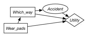
Decision nodes, drawn as rectangles, represent decision variables. The agent gets to choose a value for each decision variable. Where there are multiple decision variables, we assume there is a total ordering of the decision nodes, and the decision nodes before a decision node $D$ in the total ordering are the parents of $D$ .
•

Chance nodes, drawn as ovals, represent random variables. These are the same as the nodes in a belief network. Each chance node has an associated domain and a conditional probability of the variable, given its parents. As in a belief network, the parents of a chance node represent conditional dependence: a variable is independent of its non-descendants, given its parents. In a decision network, both chance nodes and decision nodes can be parents of a chance node.
•

A utility node, drawn as a diamond, represents the utility. The parents of the utility node are the variables on which the utility depends. Both chance nodes and decision nodes can be parents of the utility node.

Each chance variable and each decision variable has a domain. There is no domain for the utility node. Whereas the chance nodes represent random variables and the decision nodes represent decision variables, there is no utility variable.

Associated with a decision network is a conditional probability for each chance node given its parents (as in a belief network) and a utility as a function of the utility node’s parents. In the specification of the network, there are no functions associated with a decision (although the algorithm will construct a function).

Figure 9.7: Single-stage decision network for the delivery robot

$Which\_way$	$A c c i d e n t$	Value
$s h o r t$	$t r u e$	0.2
$s h o r t$	$f a l s e$	0.8
$l o n g$	$t r u e$	0.01
$l o n g$	$f a l s e$	0.99

$Wear\_pads$	$Which\_way$	$A c c i d e n t$	Utility
$t r u e$	$s h o r t$	$t r u e$	35
$t r u e$	$s h o r t$	$f a l s e$	95
$t r u e$	$l o n g$	$t r u e$	30
$t r u e$	$l o n g$	$f a l s e$	75
$f a l s e$	$s h o r t$	$t r u e$	3
$f a l s e$	$s h o r t$	$f a l s e$	100
$f a l s e$	$l o n g$	$t r u e$	0
$f a l s e$	$l o n g$	$f a l s e$	80

Example 9.10.

Figure 9.7 gives a decision network representation of Example 9.6. There are two decisions to be made: which way to go and whether to wear padding. Whether the agent has an accident only depends on which way they go. The utility depends on all three variables.

This network requires two factors: a factor representing the conditional probability, $P(Accident\mid Which\_way)$ , and a factor representing the utility as a function of $Which\_way$ , $A c c i d e n t$ , and $Wear\_pads$ . Tables for these factors are shown in Figure 9.7.

A policy for a single-stage decision network is an assignment of a value to each decision variable. Each policy has an expected utility. An optimal policy is a policy whose expected utility is maximal. That is, it is a policy such that no other policy has a higher expected utility. The value of a decision network is the expected utility of an optimal policy for the network.

1: procedure VE_SSDN(

D N

)

2: Inputs

D N

a single stage decision network

4: Output

5: An optimal policy and the expected utility of that policy.

6: Prune all nodes that are not ancestors of the utility node.

7: Sum out all chance nodes.

8: – at this stage there is a single factor

F

that was derived from utility

9: Let

v

be the maximum value in

F

10: Let

d

be an assignment that gives the maximum value

11: return

d, v

Figure 9.8: Variable elimination for a single-stage decision network

Figure 9.8 shows how variable elimination is used to find an optimal policy in a single-stage decision network. After pruning irrelevant nodes and summing out all random variables, there will be a single factor that represents the expected utility for each combination of decision variables. This factor does not have to be a factor on all of the decision variables; however, those decision variables that are not included are not relevant to the decision.

Example 9.11.

Consider running ${VE\_SSDN}$ on the decision network of Figure 9.7. No nodes are able to be pruned, so it sums out the only random variable, $A c c i d e n t$ . To do this, it multiplies both factors because they both contain $A c c i d e n t$ , and sums out $A c c i d e n t$ , giving the following factor:

$Wear\_pads$	$Which\_way$	Value
$t r u e$	$s h o r t$	$0.235+0.895=83$
$t r u e$	$l o n g$	$0.0130+0.9975=74.55$
$f a l s e$	$s h o r t$	$0.23+0.8100=80.6$
$f a l s e$	$l o n g$	$0.010+0.9980=79.2$

Thus, the policy with the maximum value – the optimal policy – is to take the short way and wear pads, with an expected utility of 83.

Artificial Intelligence 2E

9.2.1 Single-Stage Decision Networks

Example 9.10.

Example 9.11.

Artificial
Intelligence 2E