8.6.1 Sampling from a Single Variable

The simplest case is to generate the probability distribution of a single variable. This is the base case the other methods build on.

From Probabilities to Samples

To generate samples from a single discrete or real-valued variable, $X$ , first totally order the values in the domain of $X$ . For discrete variables, if there is no natural order, just create an arbitrary ordering. Given this ordering, the cumulative probability distribution is a function of $x$ , defined by $f(x)=P(X\leq x)$ .

Figure 8.27: A cumulative probability distribution

To generate a random sample for $X$ , select a random number $y$ in the domain $[0,1]$ . We select $y$ from a uniform distribution to ensure that each number between 0 and 1 has the same chance of being chosen. Let $v$ be the value of $X$ that maps to $y$ in the cumulative probability distribution. That is, $v$ is the element of $domain(X)$ such that $f(v)=y$ or, equivalently, $v=f^{-1}(y)$ . Then, $X=v$ is a random sample of $X$ , chosen according to the distribution of $X$ .

Example 8.39.

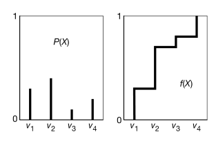
Consider a random variable $X$ with domain $\{v_{1},v_{2},v_{3},v_{4}\}$ . Suppose $P(X{=}v_{1})=0.3$ , $P(X{=}v_{2})=0.4$ , $P(X{=}v_{3})=0.1$ , and $P(X{=}v_{4})=0.2$ . First, totally order the values, say $v_{1}<v_{2}<v_{3}<v_{4}$ . Figure 8.27 shows $P(X)$ , the distribution for $X$ , and $f(X)$ , the cumulative distribution for $X$ . Consider value $v_{1}$ ; 0.3 of the domain of $f$ maps back to $v_{1}$ . Thus, if a sample is uniformly selected from the $Y$ -axis, $v_{1}$ has a 0.3 chance of being selected, $v_{2}$ has a $0.4$ chance of being selected, and so forth.

From Samples to Probabilities

Probabilities can be estimated from a set of samples using the sample average. The sample average of a proposition $\alpha$ is the number of samples where $\alpha$ is true divided by the total number of samples. The sample average approaches the true probability as the number of samples approaches infinity by the law of large numbers.

Hoeffding’s inequality provides an estimate of the error of the sample average as the probability given $n$ samples, with the guarantee of the following proposition.

Proposition 8.6 (Hoeffding).

Suppose $p$ is the true probability, and $s$ is the sample average from $n$ independent samples; then

P(\left|s-p\right|>\epsilon)\leq 2e^{-2n\epsilon^{2}}.

This theorem can be used to determine how many samples are required to guarantee a probably approximately correct estimate of the probability. To guarantee that the error is always less than some $\epsilon<0.5$ , infinitely many samples are required. However, if you are willing to have an error greater than $\epsilon$ in $\delta$ of the cases, solve $2e^{-2n\epsilon^{2}}<\delta$ for $n$ , which gives

n>\frac{-\ln\frac{\delta}{2}}{2\epsilon^{2}}.

For example, suppose you want an error less than $0.1$ , nineteen times out of twenty; that is, you are only willing to tolerate an error bigger than 0.1 in 5% of the cases. You can use Hoeffding’s bound by setting $\epsilon$ to $0.1$ and $\delta=0.05$ , which gives $n>184$ . Thus, you guarantee such bounds on the error with 185 samples. If you want an error of less than $0.01$ in at least $95\%$ of the cases, 18,445 samples could be used. If you want an error of less than $0.1$ in $99\%$ of the cases, $265$ samples could be used.

Artificial Intelligence 2E

8.6.1 Sampling from a Single Variable

From Probabilities to Samples

Example 8.39.

From Samples to Probabilities

Proposition 8.6 (Hoeffding).

Artificial
Intelligence 2E