Artificial
Intelligence 2E
foundations of computational agents
The third edition of Artificial Intelligence: foundations of computational agents, Cambridge University Press, 2023 is now available (including full text).
7.6.2 Ensemble Learning
In ensemble learning, an agent takes a number of learners and combines their predictions to make a prediction for the ensemble. The algorithms being combined are called base-level algorithms. Random forests are an example of an ensemble method, where the base-level algorithm is decision tree, and the predictions from the individual trees are averaged or are used to vote for a prediction.
In boosting, there is a sequence of learners in which each one learns from the errors of the previous ones. The features of a boosting algorithm are:
-
•
There is a sequence of base learners (that can be different from each other or the same as each other), such as small decision trees, or (squashed) linear functions
-
•
Each learner is trained to fit the examples that the previous learners did not fit well
-
•
The final prediction is a mix (e.g., sum, weighted average or mode) of the predictions of each learner.
The base learners can be weak learners, in that they do not need to be very good; they just need to better than random. These weak learners are then boosted to be components in the ensemble that performs better than any of them.
A simple boosting algorithm is functional gradient boosting which can be used for regression, as follows. The final prediction, as a function of the inputs, is the sum
where is an initial prediction, say the mean, and each is the difference from the previous prediction. Let the th prediction be . Then . Each is constructed so that the error of is minimal, given that is fixed. At each stage, the base learner learns to minimize
The th learner can learn to best fit . This is equivalent to learning from a modified data set, where the previous prediction is subtracted from the actual value of the training set. In this way, each learner is made to correct the errors of the previous prediction.
The algorithm is shown in Figure 7.19. Each is a function that, given an example, returns a prediction for that example. is a new set of examples, where for each , the latest prediction, , is subtracted from the value of the target feature . The new learner is therefore learning from the errors of the old learner. Note that does not need to be stored; the examples in can be generated as needed. The function is computed by applying the base learner to the examples .
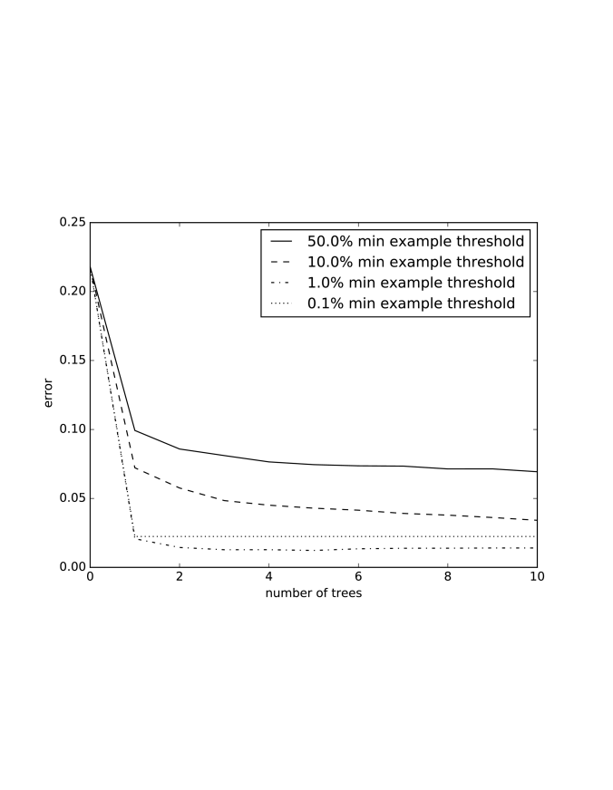
Example 7.22.
Figure 7.20 shows a plot of the sum-of-squares error as the number of trees increases for functional gradient boosting of decision trees. The different lines are for different thresholds for the minimum number of examples required for a split, as a proportion of the total examples. At one tree, it is just the decision tree algorithm. Boosting makes the tree with a 1% threshold eventually better than with a 0.1% threshold, even though they are about the same for a single tree. The code is available from the book website.