Artificial
Intelligence 2E
foundations of computational agents
The third edition of Artificial Intelligence: foundations of computational agents, Cambridge University Press, 2023 is now available (including full text).
4.7.4 Evaluating Randomized Algorithms
It is difficult to compare randomized algorithms when they give a different result and a different run time each time they are run, even for the same problem. It is especially difficult when the algorithms sometimes do not find an answer; they either run forever or must be stopped at an arbitrary point.
Unfortunately, summary statistics, such as the mean or median run time, are not very useful. For example, comparing algorithms on the mean run time requires deciding how to average in unsuccessful runs, where no solution was found. If unsuccessful runs are ignored in computing the average, an algorithm that picks a random assignment and then stops would be the best algorithm; it does not succeed very often, but when it does, it is very fast. Treating the non-terminating runs as having infinite time means all algorithms that do not find a solution will have infinite averages. A run that has not found a solution will need to be terminated. Using the time it was terminated in the average is more of a function of the stopping time than of the algorithm itself, although this does allow for a crude trade-off between finding some solutions fast versus finding more solutions.
If you were to compare algorithms using the median run time, you would prefer an algorithm that solves the problem 51% of the time but very slowly over one that solves the problem 49% of the time but very quickly, even though the latter is more useful. The problem is that the median (the 50th percentile) is just an arbitrary value; you could just as well consider the 47th percentile or the 87th percentile.
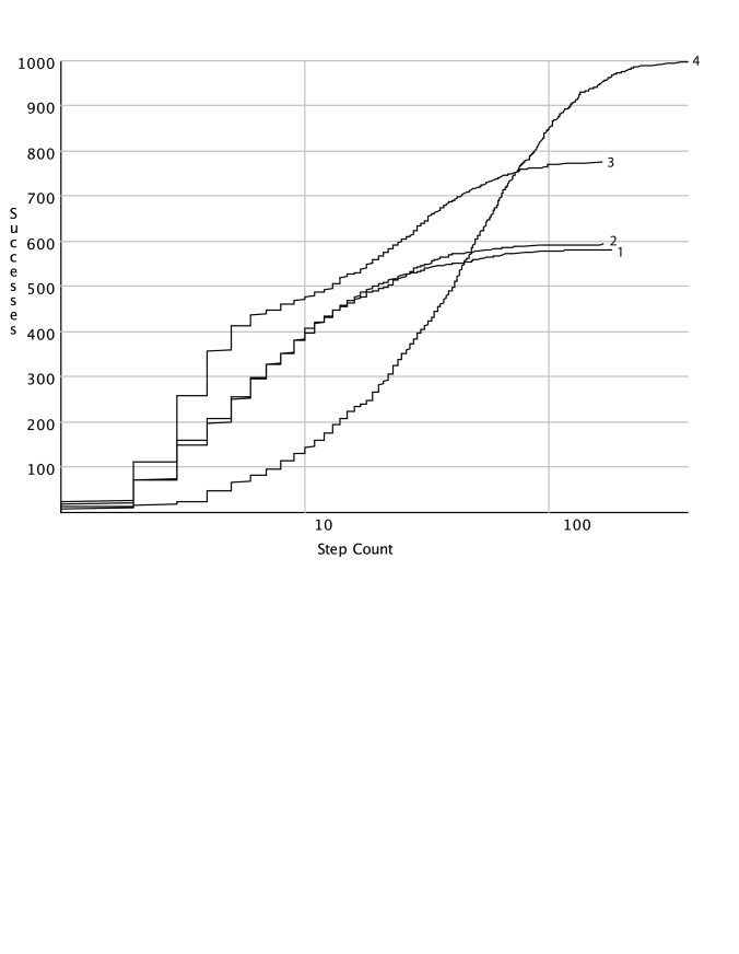
One way to visualize the run time of an algorithm for a particular problem is to use a run-time distribution, which shows the variability of the run time of a randomized algorithm on a single problem instance. The -axis represents either the number of steps or the run time. The -axis shows, for each value of , the number of runs, or proportion of the runs, solved within that run time or number of steps. Thus, it provides a cumulative distribution of how often the problem was solved within some number of steps or run time. For example, you can find the run time of the 30th percentile of the runs by finding the -value that maps to 30% on the -scale. The run-time distribution can be plotted (or approximated) by running the algorithm for a large number of times (say, 100 times for a rough approximation or 1000 times for a reasonably accurate plot) and then by sorting the runs by run time.
Example 4.24.
Four empirically generated run-time distributions for a single problem are shown in Figure 4.10. On the -axis is the number of steps, using a logarithmic scale. On the -axis is the number of instances that were successfully solved out of 1000 runs. This shows four run-time distributions on the same problem instance. Algorithms 1 and 2 solved the problem 40% of the time in 10 or fewer steps. Algorithm 3 solved the problem in about 50% of the runs in 10 or fewer steps. Algorithm 4 found a solution in 10 or fewer steps in about 12% of the runs. Algorithms 1 and 2 found a solution in about 58% of the runs. Algorithm 3 could find a solution about 80% of the time. Algorithm 4 always found a solution. This only compares the number of steps; the time taken would be a better evaluation but is more difficult to measure for small problems and depends on the details of the implementation.
One algorithm strictly dominates another for this problem if its run-time distribution is completely to the left (and above) the run-time distribution of the second algorithm. Often two algorithms are incomparable under this measure. Which algorithm is better depends on how much time an agent has before it needs to use a solution or how important it is to actually find a solution.
Example 4.25.
In the run-time distributions of Figure 4.10, Algorithm 3 dominates Algorithms 1 and 2. Algorithms 1 and 2 are actually different sets of runs of the same algorithm with the same settings. This shows the errors that are typical of multiple runs of the same stochastic algorithm on the same problem instance. Algorithm 3 is better than Algorithm 4 up to 60 steps, after which Algorithm 4 is better.
By looking at the graph, you can see that Algorithm 3 often solves the problem in its first four or five steps, after which it is not as effective. This may lead you to try to suggest using Algorithm 3 with a random restart after five steps and this does, indeed, dominate all of the algorithms for this problem instance, at least in the number of steps (counting a restart as a single step). However, because the random restart is an expensive operation, this algorithm may not be the most efficient. This also does not necessarily predict how well the algorithm will work in other problem instances.