Artificial
Intelligence 2E
foundations of computational agents
The third edition of Artificial Intelligence: foundations of computational agents, Cambridge University Press, 2023 is now available (including full text).
4.3 Solving CSPs Using Search
Generate-and-test algorithms assign values to all variables before checking the constraints. Because individual constraints only involve a subset of the variables, some constraints can be tested before all of the variables have been assigned values. If a partial assignment is inconsistent with a constraint, any total assignment that extends the partial assignment will also be inconsistent.
Example 4.11.
In the delivery scheduling problem of Example 4.9, the assignments and are inconsistent with the constraint regardless of the values of the other variables. If the variables and are assigned values first, this inconsistency can be discovered before any values are assigned to , , or , thus saving a large amount of work.
An alternative to generate-and-test algorithms is to construct a search space for the search strategies of the previous chapter to use. The graph to search is defined as follows:
-
•
The nodes are assignments of values to some subset of the variables.
-
•
The neighbors of a node are obtained by selecting a variable that is not assigned in node and by having a neighbor for each assignment of a value to that does not violate any constraint.
Suppose node is the assignment . To find the neighbors of , select a variable that is not in the set . For each value , where is consistent with each of the constraints, the node is a neighbor of .
-
•
The start node is the empty assignment that does not assign a value to any variables.
-
•
A goal node is a node that assigns a value to every variable. Note that this only exists if the assignment is consistent with all of the constraints.
In this case, it is not the path from the start node that is of interest, but the goal nodes.
Example 4.12.
Suppose you have a very simple CSP with the variables , , and , each with domain . Suppose the constraints are and . A possible search tree is shown in Figure 4.1.
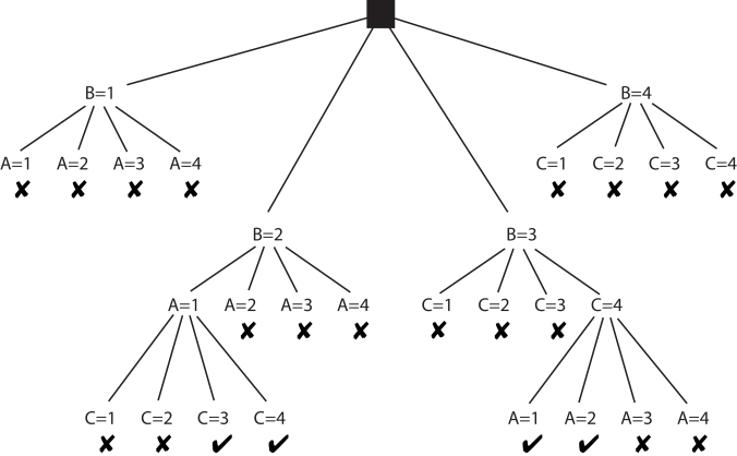
In this figure, a node corresponds to all of the assignments from the root to that node. The potential nodes that are pruned because they violate constraints are labeled with ✘.
The leftmost ✘ corresponds to the assignment , . This violates the constraint, and so it is pruned.
This CSP has four solutions. The leftmost one is , , . The size of the search tree, and thus the efficiency of the algorithm, depends on which variable is selected at each time. A static ordering, such as always splitting on then then , is usually less efficient than the dynamic ordering used here, but it might be more difficult to find the best dynamic ordering than to find the best static ordering. The set of answers is the same regardless of the variable ordering.
There would be total assignments tested in a generate-and-test algorithm. For the search method, there are 8 total assignments generated, and 16 other partial assignments that were tested for consistency.
Searching this tree with a depth-first search, typically called backtracking, can be much more efficient than generate and test. Generate and test is equivalent to not checking constraints until reaching the leaves. Checking constraints higher in the tree can prune large subtrees that do not have to be searched.