Artificial
Intelligence 2E
foundations of computational agents
The third edition of Artificial Intelligence: foundations of computational agents, Cambridge University Press, 2023 is now available (including full text).
12.6 Evaluating Reinforcement Learning Algorithms
We can judge a reinforcement learning algorithm either by how good a policy it finds or by how much reward it receives while acting and learning. Which is more important depends on how the agent will be deployed. If there is sufficient time for the agent to learn safely before it is deployed, the final policy may be the most important. If the agent has to learn while being deployed, it may never get to the stage where it no longer need to explore, and the agent needs to maximize the reward it receives while learning.
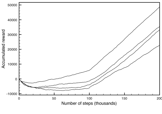
One way to show the performance of a reinforcement learning algorithm is to plot the cumulative reward (the sum of all rewards received so far) as a function of the number of steps. One algorithm dominates another if its plot is consistently above the other.
Example 12.4.
Figure 12.4 compares four runs of the Q-learner on the game of Example 12.2.
The plots are for different runs that varied according to whether was fixed, according to the initial values of the -function, and according to the randomness in the action selection. They all used greedy exploit of 80% (i.e., ) for the first 100,000 steps, and 100% (i.e., ) for the next 100,000 steps. The top plot dominated the others.
There can be a great deal of variability of each algorithm on different runs, so to actually compare these algorithms the same algorithm must be run multiple times.
There are three statistics of this plot that are important:
-
•
The asymptotic slope shows how good the policy is after the algorithm has stabilized.
-
•
The minimum of the curve shows how much reward must be sacrificed before it starts to improve.
-
•
The zero crossing shows how long it takes until the algorithm has recouped its cost of learning.
The last two statistics are applicable when both positive and negative rewards are available and having these balanced is reasonable behavior. For other cases, the cumulative reward should be compared with reasonable behavior that is appropriate for the domain; see Exercise 2.
It is also possible to plot the average reward (the accumulated reward per time step). This more clearly shows the value of policy eventually learned and whether the algorithm has stopped learning (when it is flat), but often has large variations for early times.
One thing that should be noted about the cumulative reward plot is that it measures total reward, yet the algorithms optimize discounted reward at each step. In general, you should optimize for, and evaluate your algorithm using, the optimality criterion that is most appropriate for the domain.