Artificial
Intelligence 2E
foundations of computational agents
The third edition of Artificial Intelligence: foundations of computational agents, Cambridge University Press, 2023 is now available (including full text).
12.10.2 Learning to Coordinate
Dimensions: flat, states, finite horizon, partially observable, stochastic, utility, learning, multiple agents, online, perfect rationality
For multiple agents with imperfect information, including simultaneous action games, it is possible that there are multiple Nash equilibria, and that no deterministic strategy is optimal. Due to the existence of multiple equilibria, in many cases it is not clear what an agent should actually do, even if it knows all of the outcomes for the game and the utilities of the agents. However, most real strategic encounters are much more difficult, because the agents do not know the outcomes or the utilities of the other agents.
For games where the only Nash equilibria consist of randomized strategies, such as in the soccer penalty kick (Figure 11.7), learning any deterministic policy is not a good idea because any deterministic strategy can be exploited by the other agent. For other games with multiple Nash equilibria, such as those explored in Section 11.4, agents may need to play multiple games to coordinate on a strategy profile where neither want to deviate.
Reinforcement learning can be extended to such situations by explicitly representing stochastic policies, which are policies that specify a probability distribution over actions. This automatically allows for a form of exploration, because any action with a non-zero probability will be tried repeatedly.
This section presents a simple algorithm to iteratively improve an agent’s policy. The agents repeatedly play the same game. Each agent plays a stochastic strategy; the agent updates the probabilities of its actions based on the payoffs received. For simplicity, it only has a single state; the only thing that changes between times is the randomized policies of the other agents.
The policy hill-climbing controller of Figure 12.8 keeps updating its probability of the best action based on experience. The inputs are the set of actions, a step size for changing the estimate of , a step size for changing the randomness of the policy. is the number of actions (the number of elements of ).
A stochastic policy is a probability distribution over actions. The algorithm maintains its current stochastic policy in the array and an estimate of the payoff for each action in the array. The agent carries out an action based on its current policy and observes the action’s payoff. It then updates its estimate of the value of that action and modifies its current strategy by increasing the probability of its best action.
The algorithm initializes randomly so that it is a probability distribution; is initialized arbitrarily.
At each stage, the agent selects an action according to the current distribution . It carries out the action and observes the payoff it receives. It then updates its estimate of , using the temporal difference equation (12.1) LABEL:1TD-eqn.
It then computes , which is the current best action according to its estimated -values. (Assume that, if there is more than one best action, one is chosen at random to be .) It reduces the probability of the other actions by , ensuring that the probabilities never become negative. The probability of is made to ensure all probabilities sum to 1. Note that if none of the probabilities of the other actions became negative (and needed to be adjusted back to 0), the probability of is increased by .
This algorithm needs to trade off exploration and exploitation. One way to do this is to use an -greedy exploration strategy, which the following examples use with the explore probability of 0.05. An alternative is to make sure that the probability of any action never gets less than some threshold.
Open-source implementations of this learning controller are available from the book’s website.
Example 12.8.
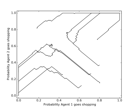
Figure 12.9 shows a plot of the learning algorithm for the football–shopping game of Example 11.12. This figure plots the probabilities for Agent 1 choosing shopping and Agent 2 choosing shopping for eight runs of the learning algorithm. Each line is one run. Each of the runs ends at the top-right corner or the bottom-left corner, where the agents have learned to coordinate. In these runs, the policies are initialized randomly, , and .
If the other agents are playing a fixed strategy (even if it is a stochastic strategy), this algorithm converges to a best response to that strategy (as long as and are small enough, and as long as the agent randomly tries all of the actions occasionally).
The following discussion assumes that all agents are using this learning controller.
If there is a unique Nash equilibrium in pure strategies, and all of the agents use this algorithm, they will converge to this equilibrium. Dominated strategies will have their probability set to zero. In Example 11.15, it will find the Nash equilibrium. Similarly for the prisoner’s dilemma in Example 11.13, it will converge to the unique equilibrium where both agents take. Thus, this algorithm does not learn to cooperate, where cooperating agents will both give in the prisoner’s dilemma to maximize their payoffs.
If there are multiple pure equilibria, this algorithm will converge to one of them. The agents thus learn to coordinate. For example, in the football–shopping game of Example 11.12, it will converge to one of the equilibria of both shopping or both going to the football game, as shown in Figure 12.9. Which one it converges to depends on the initial strategies.
If there is only a randomized equilibrium, as in the penalty kick game of Example 11.9, this algorithm tends to cycle around the equilibrium.
Example 12.9.
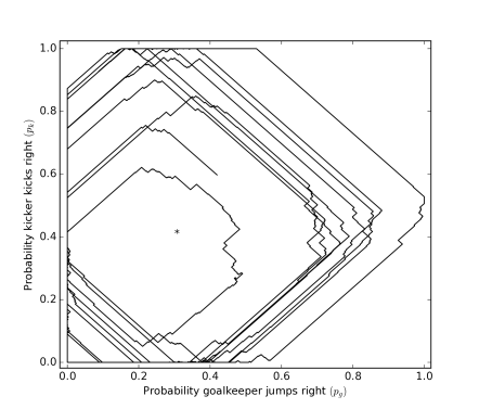
Figure 12.10 shows a plot of two players using the learning algorithm for Example 11.9. This figure plots the probabilities for the goalkeeper jumping right and the kicker kicking right for one run of the learning algorithm. In this run, and . The learning algorithm cycles around the equilibrium never actually reaching the equilibrium. At equilibrium, marked with * in the figure, the kicker kicks right with probability 0.4 and the goalkeeper jumps right with probability 0.3 (see Example 11.16).
Consider a two-agent competitive game where there is only a randomized Nash equilibrium. If agent is playing agent and agent is playing a Nash equilibrium, it does not matter which action in its support set is performed by agent ; they all have the same value to . Thus, agent will tend to wander off the equilibrium. Note that, when deviates from the equilibrium strategy, the best response for agent is to play deterministically. This algorithm, when used by agent , eventually notices that has deviated from the equilibrium and agent changes its policy. Agent will also deviate from the equilibrium. Then agent can try to exploit this deviation. When they are both using this controller, each agents’s deviation can be exploited, and they tend to cycle.
There is nothing in this algorithm to keep the agents on a randomized equilibrium. One way to try to make agents not wander too far from an equilibrium is to adopt a win or learn fast (WoLF) strategy: when the agent is winning it takes small steps ( is small), and when the agent is losing it takes larger steps ( is increased). While it is winning, it tends to stay with the same policy, and while it is losing, it tries to move quickly to a better policy. To define winning, a simple strategy is for an agent to see whether it is doing better than the average payoff it has received so far.
Note that there is no perfect learning strategy. If an opposing agent knew the exact strategy (whether learning or not) agent was using, and could predict what agent would do, it could exploit that knowledge.